Promising Different to Multi-Layer Perceptron?

A brand new machine studying paper dropped by that boldly presents a brand new path within the deep-learning discipline. The current publication on Kolmogorov-Arnold Networks (KANs) is exactly a kind of groundbreaking works. Right this moment, we’ll attempt to perceive this paper’s concepts and basic ideas of KANs.

A brand new machine-learning algorithm, Kolmogorov-Arnold Networks (KANs) guarantees to be an alternative choice to Multi-Layer Perceptron. Multi-layer perceptrons (MLPs), or fully-connected feedforward neural networks, are just like the foundational blocks of recent deep studying. They’re necessary for tackling complicated issues as a result of they’re good at approximating curved relationships between enter and output information.

That will help you perceive KANs higher, we’ve got added a pocket book demo utilizing Paperspace. Paperspace GPUs excel at parallel computing, effectively dealing with hundreds of simultaneous operations, making them splendid for duties like deep studying and information evaluation. Switching to Paperspace companies supplies scalable, on-demand entry to highly effective {hardware}, eliminating the necessity for important upfront investments and upkeep.

However, are they the final word resolution for constructing fashions that perceive and predict issues?

Regardless of their widespread use, MLPs do have some downsides. As an illustration, in fashions like transformers, MLPs deplete a number of the parameters that are not concerned in embedding information. Plus, they’re typically obscure making them a black field mannequin, in comparison with different components of the mannequin, like consideration layers, which may make it tougher to determine why they make sure predictions with out extra evaluation instruments.

Why is it thought of as an alternative choice to MLP?

Whereas MLPs are all about mounted activation features on nodes, KANs flip the script by placing learnable activation features on the sides. This implies every weight parameter in a KAN is changed by a learnable 1D operate, making the community extra versatile. Surprisingly, regardless of this added complexity, KANs typically require smaller computation graphs than MLPs. In reality, in some instances, a less complicated KAN can outperform a a lot bigger MLP each in accuracy and parameter effectivity, like in fixing partial differential equations (PDE).

Different analysis papers have additionally tried to use this theorem to coach machine studying fashions previously. Nevertheless, this specific paper takes a step additional by increasing the concept. It introduces a extra generalized method in order that we are able to practice neural networks of any dimension and complexity utilizing backpropagation.

What’s KAN?

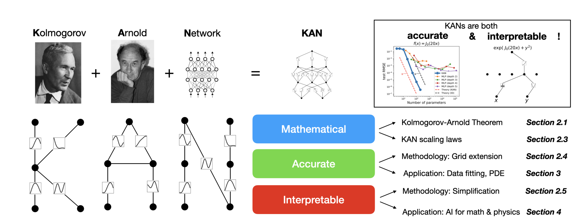
KANs are based mostly on the Kolmogorov-Arnold illustration theorem,

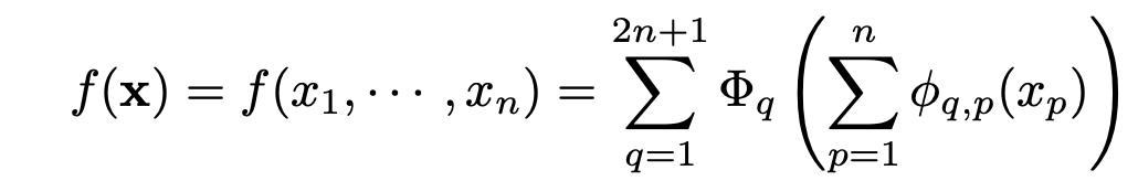
To grasp this, allow us to take an instance of a multivariate equation like this,

This can be a multivariate operate as a result of right here, y relies upon upon x1, x2, …xn.
In line with the theory, we are able to categorical this as a mix of single-variable features. This permits us to interrupt down the multivariable equation into a number of particular person equations, every involving one variable and one other operate of it, and so forth. Then sum up the outputs of all of those features and move that sum by yet one more univariate operate, f as proven right here.

Additional, as an alternative of creating one composition, we do a number of compositions, reminiscent of m completely different compositions and sum them up.

Additionally, We are able to rewrite the above equation to,

Overview of the Paper

The paper demonstrated that addition is the one true multivariate operate, as each different operate will be expressed by a mix of univariate features and summation. At first look, this would possibly seem to be a breakthrough for machine studying, lowering the problem of studying high-dimensional features to mastering a polynomial variety of 1D features.
In less complicated phrases, it is like saying that even when coping with an advanced equation or a machine studying process the place the result depends upon many components, we are able to break it down into smaller, easier-to-handle components. We give attention to every issue individually, kind of like fixing one piece of the puzzle at a time, after which put all the pieces collectively to resolve the larger drawback. So, the principle problem turns into determining tips on how to cope with these particular person components, which is the place machine studying and methods like backpropagation step in to assist us out.

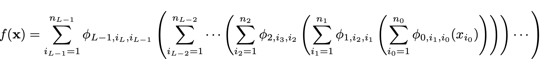
The unique Kolmogorov-Arnold illustration equation aligns with a 2-layer KAN having a form of [n, 2n + 1, 1].

It is value noting that each one operations inside this illustration are differentiable, enabling us to coach KANs utilizing backpropagation.

The above equation exhibits that the outer sum loops by all the completely different compositions from 1 to m. Additional, the inside sum loops by every enter variable x1 to xn for every outer operate q. In matrix kind, this may be represented beneath.

Right here, the inside operate will be depicted as a matrix stuffed with numerous activation features (denoted as phi). Moreover, we’ve got an enter vector (x) with n options, which is able to traverse by all of the activation features. Please word right here that phi represents because the activation operate and never the weights. These activation features are referred to as B-Splines. So as to add right here every of those features are easy polynomial curves. The curves rely upon the enter of x.

Visible Illustration of KAN

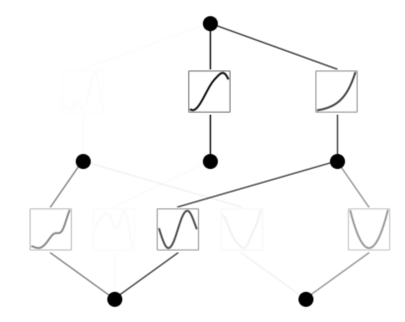
Here’s a visible illustration of coaching a 3-layer KAN,

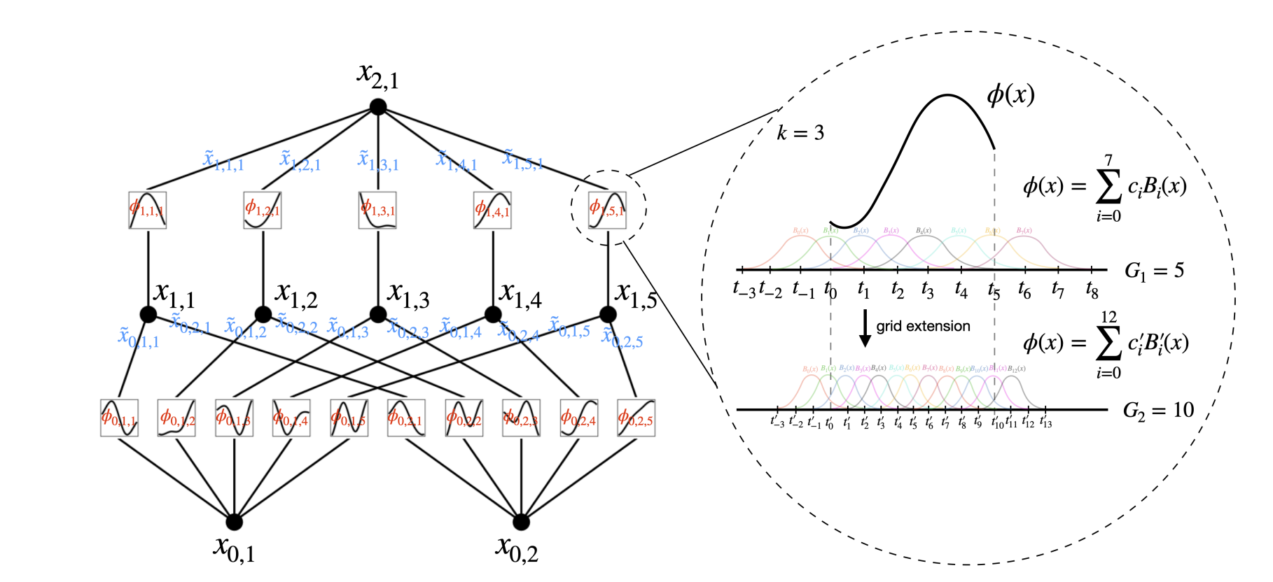
Within the given illustration, there are two enter options and a primary output layer consisting of 5 nodes. Every output from these nodes undergoes 5 distinct parameterized univariate activation features. The ensuing activations are then summed to yield the options for every output node. This whole course of constitutes a single KAN layer with an enter dimension of two and an output dimension of 5. Like multi-layer perceptron (MLP), a number of KAN layers will be stacked on prime of one another to generate an extended, deeper neural community. The output of 1 layer is the enter to the following. Additional, like MLPs, the computation graph is absolutely differentiable, because it depends on differentiable activation features and summation on the node stage, enabling coaching through backpropagation and gradient descent.

Distinction between MLPs and KANs

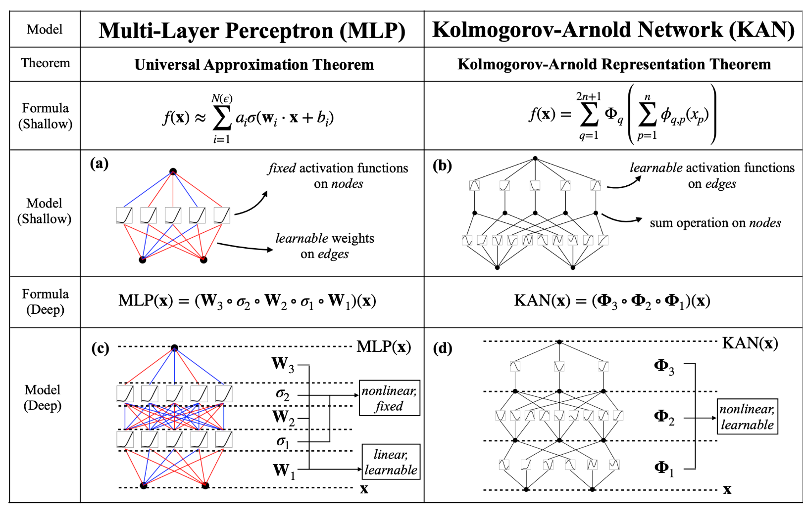
One key differentiator between the 2 networks is that MLPs place mounted activation features on the nodes. In distinction, KANs place learnable activation features alongside the sides, and the nodes sum it up.

In MLPs, activation features are parameter-free and carry out mounted operations on inputs, whereas learnable parameters are simply linear weights and biases. In distinction, KANs lack linear weight matrices totally; as an alternative, every weight parameter is substituted with a learnable non-linear activation operate.
Additionally, contemplating the instability situation with conventional activation features in neural networks makes coaching fairly difficult. To handle this, the authors of KANs make use of B-splines, which supply higher stability and bounded habits.

B-Splines

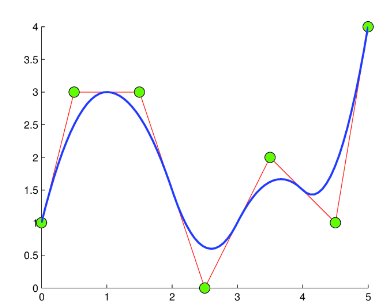
Now, let’s perceive B-splines briefly. B-splines are primarily curves made up of polynomial segments, every with a specified stage of smoothness. Image every phase as a small curve, the place a number of management factors affect the form. In contrast to less complicated spline curves, which depend on solely two management factors per phase, B-splines use extra, resulting in smoother and extra adaptable curves.

The magic of B-splines lies of their native affect. Adjusting one management level impacts solely the close by part of the curve, leaving the remainder undisturbed. This property gives outstanding benefits, particularly in sustaining smoothness and facilitating differentiability, which is essential for efficient backpropagation throughout coaching.

Coaching KANs

Backpropagation is an important method for decreasing the loss in machine studying. It’s essential for coaching neural networks by iteratively adjusting their parameters based mostly on noticed errors. In KANs, backpropagation is important for fine-tuning community parameters, together with edge weights and coefficients of learnable activation features.

Coaching KANs start with the random initialization of community parameters. The community then undergoes ahead and backward passes: enter information is fed by the community to generate predictions, that are in comparison with precise labels to calculate loss. Backpropagation computes gradients of the loss with respect to every parameter utilizing the chain rule of calculus. These gradients information the parameter updates by strategies like gradient descent, stochastic gradient descent, or Adam optimization.

A key problem in coaching KANs is making certain stability and convergence throughout optimization. Researchers use methods reminiscent of dropout and weight decay for regularization and punctiliously choose optimization algorithms and studying charges to handle this. Moreover, batch normalization and layer normalization methods assist stabilize coaching and speed up convergence.

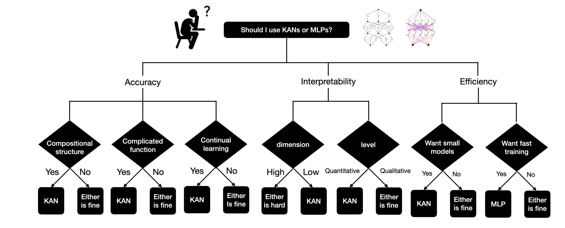
KANs or MLPs?

The primary disadvantage of KANs is their sluggish coaching velocity, which is about 10 occasions slower than MLPs with the identical variety of parameters. Nevertheless, the analysis has not but targeted a lot on optimizing KANs’ effectivity, so there’s nonetheless scope for enchancment. If you happen to want quick coaching, go for MLPs. However in case you prioritize interpretability and accuracy, and do not thoughts slower coaching, KANs are value a attempt.

The important thing differentiators between MLPs and KANs are:

(i) Activation features are on edges as an alternative of on nodes,

(ii) Activation features are learnable as an alternative of mounted.

Benefits of KAN’s

• KAN’s can be taught their activation features, thus making them extra expressive than customary MLPs, and capable of be taught features with fewer parameters.
• Additional, the paper exhibits that KANs outperform MLPs utilizing considerably fewer parameters.
• A way referred to as grid extension permits for fine-tuning KANs by making the spline management grids finer, rising accuracy with out retraining from scratch. This provides extra parameters to the mannequin for increased variance and expressiveness.
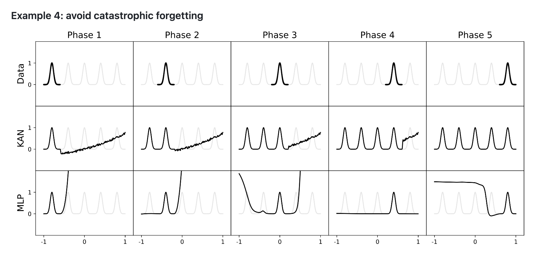
• KANs are much less susceptible to catastrophic forgetting as a consequence of B-splines’ native management.
  • Catastrophic forgetting happens when a educated neural community forgets earlier coaching upon fine-tuning with new information.
  • In MLPs, weights change globally, inflicting the community to neglect previous information when studying new information.
  • In KANs, adjusting management factors of splines impacts solely native areas, preserving earlier coaching.
• The paper comprises many different fascinating insights and methods associated to KANs; therefore, we extremely suggest that our readers learn it.

Get KANs working

Set up through github:

!pip set up git+https://github.com/KindXiaoming/pykan.git

Set up through PyPI:

!pip set up pykan

Necessities:

# python==3.9.7
matplotlib==3.6.2
numpy==1.24.4
scikit_learn==1.1.3
setuptools==65.5.0
sympy==1.11.1
torch==2.2.2
tqdm==4.66.2

Initialize KAN and create a KAN,

from kan import *
# create a KAN: 2D inputs, 1D output, and 5 hidden neurons. cubic spline (ok=3), 5 grid intervals (grid=5).
mannequin = KAN(width=[2,5,1], grid=5, ok=3, seed=0)

# create dataset f(x,y) = exp(sin(pi*x)+y^2)
f = lambda x: torch.exp(torch.sin(torch.pi*x[:,[0]]) + x[:,[1]]**2)
dataset = create_dataset(f, n_var=2)
dataset['train_input'].form, dataset['train_label'].form

# plot KAN at initialization
mannequin(dataset['train_input']);
mannequin.plot(beta=100)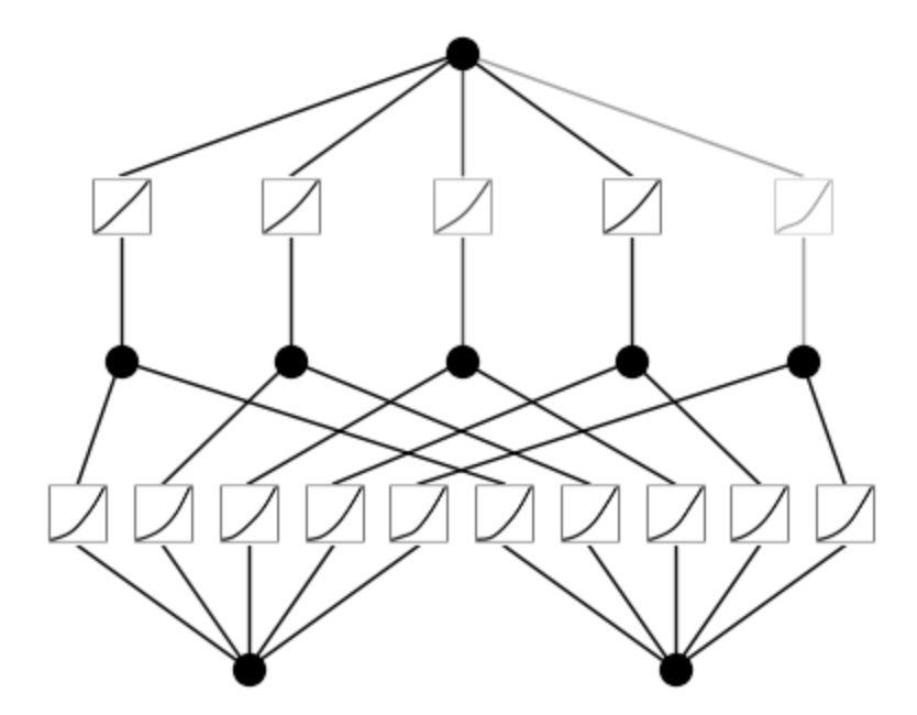

# practice the mannequin
mannequin.practice(dataset, choose="LBFGS", steps=20, lamb=0.01, lamb_entropy=10.);

mannequin.plot()

mannequin.prune()
mannequin.plot(masks=True)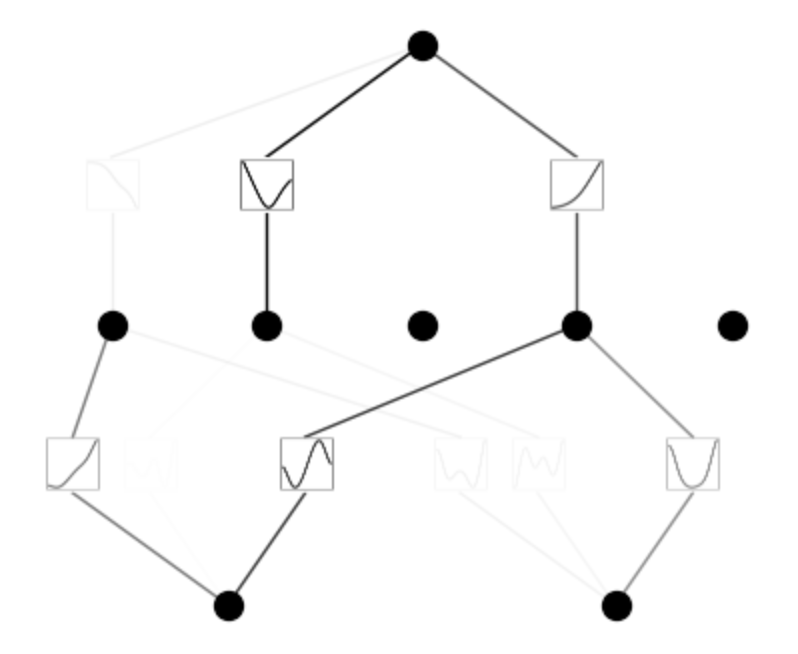

mannequin = mannequin.prune()
mannequin(dataset['train_input'])
mannequin.plot()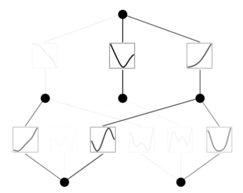

mannequin.practice(dataset, choose="LBFGS", steps=50);

practice loss: 2.09e-03 | check loss: 2.17e-03 | reg: 1.64e+01 : 100%|██| 50/50 [00:20<00:00, 2.41it/s]

mannequin.plot()

mode = "auto" # "guide"

if mode == "guide":
    # guide mode
    mannequin.fix_symbolic(0,0,0,'sin');
    mannequin.fix_symbolic(0,1,0,'x^2');
    mannequin.fix_symbolic(1,0,0,'exp');
elif mode == "auto":
    # computerized mode
    lib = ['x','x^2','x^3','x^4','exp','log','sqrt','tanh','sin','abs']
    mannequin.auto_symbolic(lib=lib)

fixing (0,0,0) with log, r2=0.9692028164863586
fixing (0,0,1) with tanh, r2=0.6073551774024963
fixing (0,0,2) with sin, r2=0.9998868107795715
fixing (0,1,0) with sin, r2=0.9929550886154175
fixing (0,1,1) with sin, r2=0.8769869804382324
fixing (0,1,2) with x^2, r2=0.9999980926513672
fixing (1,0,0) with tanh, r2=0.902226448059082
fixing (1,1,0) with abs, r2=0.9792929291725159
fixing (1,2,0) with exp, r2=0.9999933242797852

mannequin.practice(dataset, choose="LBFGS", steps=50);

practice loss: 1.02e-05 | check loss: 1.03e-05 | reg: 1.10e+03 : 100%|██| 50/50 [00:09<00:00, 5.22it/s]

Abstract of KANs’ Limitations and Future Instructions

As per the analysis we have discovered that KANs outperform MLPs in scientific duties like becoming bodily equations and fixing PDEs. They present promise for complicated issues reminiscent of Navier-Stokes equations and density useful principle. KANs may additionally improve machine studying fashions, like transformers, doubtlessly creating “kansformers.”

KANs excel as a result of they convey within the “language” of science features. This makes them splendid for AI-scientist collaboration, enabling simpler and simpler interplay between AI and researchers. As an alternative of aiming for absolutely automated AI scientists, growing AI that assists scientists by understanding their particular wants and preferences is extra sensible.

Additional, important considerations should be addressed earlier than KANs can doubtlessly exchange MLPs in machine studying. The primary situation is that KANs cannot make the most of GPU parallel processing, stopping them from benefiting from the fast-batched matrix multiplications that GPUs supply. This limitation means KANs practice very slowly since their completely different activation features cannot effectively leverage batch computation or course of a number of information factors in parallel. Therefore, if velocity is essential, MLPs are higher. Nevertheless, in case you prioritize interpretability and accuracy and might tolerate slower coaching, KANs are a sensible choice.

Moreover, the authors have not examined KANs on massive machine-learning datasets, so it is unclear if they provide any benefit over MLPs in real-world eventualities.

We hope you discovered this text fascinating. We extremely suggest checking the sources part for extra info on KANs.

Thanks!

Sources