Constructing Interactive Knowledge Visualizations with D3.js and React — SitePoint

Knowledge visualizations are a strong technique to signify advanced info in a digestible and interesting method. React, a preferred JavaScript library for constructing consumer interfaces, could be built-in with D3.js to create beautiful and interactive knowledge visualizations.

This information will stroll by means of constructing knowledge visualizations in React utilizing D3.js. From understanding how D3.js works and methods to combine it with React to crafting an interactive world inhabitants dashboard, every part of this information will present complete insights and sensible examples.

The picture beneath exhibits a sneak peek at our ultimate product.

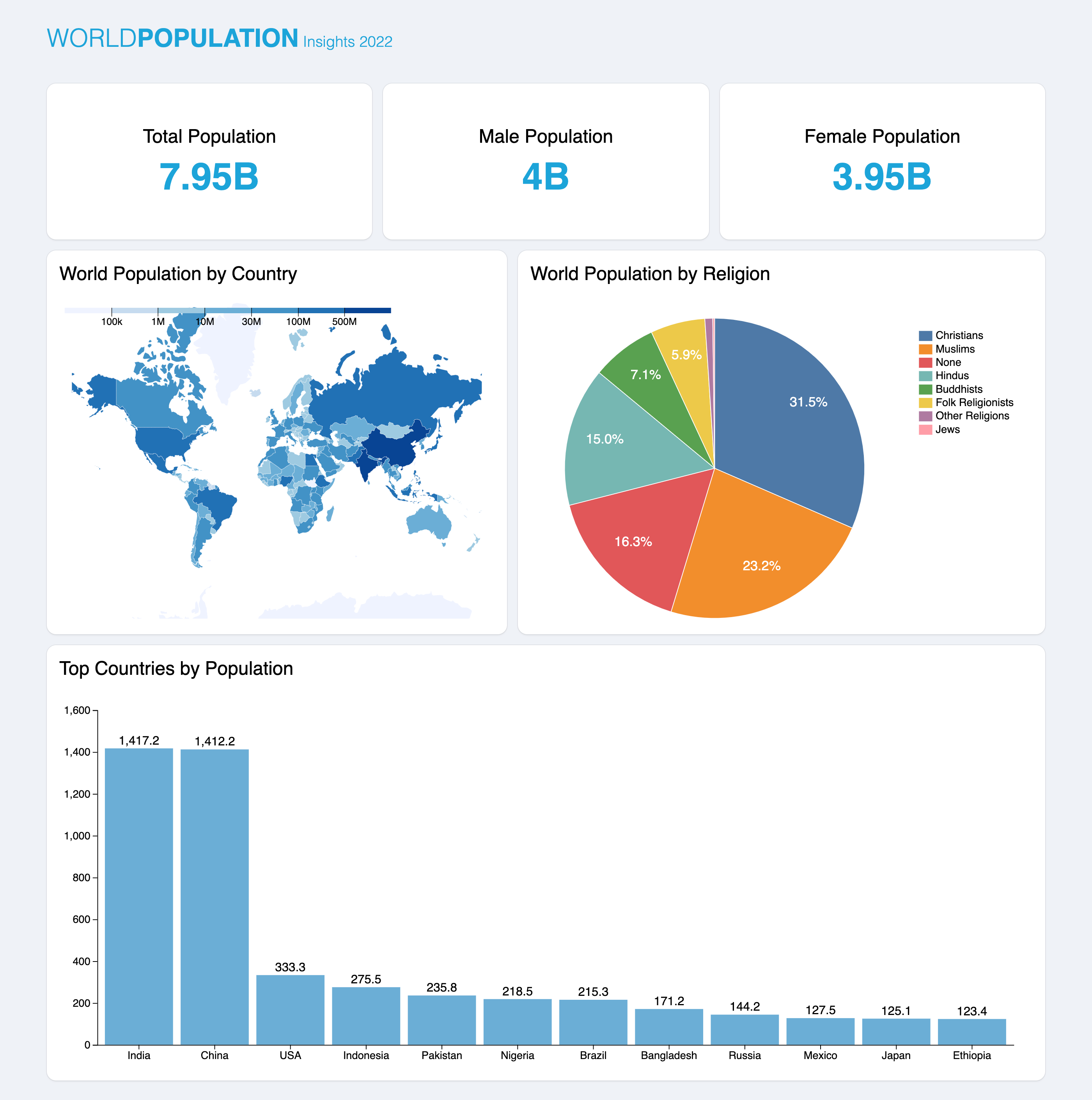
You possibly can take a look at the stay demo and discover the whole supply code on GitHub.

Let’s get began!

Stipulations

Earlier than we delve into this information, it’s important to have a fundamental understanding of React. Should you’re new to React, think about reviewing the official documentation and finishing a couple of introductory tutorials. Familiarity with JavaScript and ES6 syntax can even be useful.

Understanding D3.js and React Integration

D3.js, or Knowledge-Pushed Paperwork, is a JavaScript library that facilitates the creation of visualizations within the browser. Its core energy lies in binding knowledge to the doc object mannequin (DOM) and making use of data-driven transformations to the doc. It additionally operates on normal net applied sciences like HTML, CSS, and SVG, making it an excellent companion for React functions.

Benefits of utilizing D3.js with React

• Wealthy set of options. D3.js gives complete options for creating varied visualizations, from easy bar charts to advanced hierarchical visualizations. Its versatility makes it a go-to selection for data-driven functions.

• Part reusability. React’s component-based construction permits for creating reusable visualization parts. When you’ve crafted a D3.js-powered element, you possibly can simply combine it into totally different components of your utility.

• Environment friendly state administration. React’s state administration ensures that your visualizations replace seamlessly in response to adjustments within the underlying knowledge. This characteristic is especially helpful for real-time functions.

Putting in D3.js and React

Getting began with D3.js in your React apps is a breeze. You possibly can start by creating a brand new React venture utilizing Vite:

npm create vite@newest react-d3-demo -- --template react


yarn create vite react-d3-demo --template react

As soon as your venture is about up, set up D3.js utilizing npm or Yarn:

npm set up d3


yarn add d3

Deciding on and modifying parts in D3.js

Earlier than delving into constructing visualizations, we should take a look at some elementary ideas in D3. The primary idea we’ll study is choosing and modifying parts with D3.js. This course of entails figuring out parts within the DOM and modifying their properties.

Let’s take a look at an instance beneath:

import { useEffect } from "react";
import * as d3 from "d3";

perform App() {
  useEffect(() => {
    
    d3.choose("p").textual content("Good day, D3.js!");
  }, []);

  return <p></p>;
}

export default App;

Within the code above, we choose the <p> factor utilizing D3’s choose() technique. This technique selects the primary factor within the DOM that matches the desired selector.

After choosing the factor, we modify it utilizing the textual content() technique that adjustments the textual content content material of the chosen paragraph to “Good day, D3.js!”.

When coping with visualizations the place a number of parts signify totally different knowledge factors, choosing only one factor may not be adequate. That is the place D3’s selectAll() technique comes into play. Not like choose(), which picks the primary matching factor, selectAll() grabs all parts that match the desired selector:

import { useEffect } from "react";
import * as d3 from "d3";

perform App() {
  useEffect(() => {
    d3.selectAll(".textual content").fashion("coloration", "skyblue").textual content("Good day, D3.js!");
  }, []);

  return (
    <div className="texts">
      <p className="textual content"></p>
      <p className="textual content"></p>
      <p className="textual content"></p>
      <p className="textual content"></p>
    </div>
  );
}

export default App;

Becoming a member of knowledge in D3.js

D3.js employs an information be a part of idea to synchronize knowledge with DOM parts. Think about the next instance:

import { useEffect } from "react";
import * as d3 from "d3";

perform App() {
  useEffect(() => {
    const knowledge = [10, 20, 30, 40, 50];

    
    const circles = d3
      .choose("svg")
      .attr("width", "100%")
      .attr("peak", "100%");

    
    circles
      .selectAll("circle")
      .knowledge(knowledge)
      .be a part of("circle")
      .attr("cx", (d, i) => i * d + (3 * d + 20))
      .attr("cy", 100)
      .attr("r", (d) => d)
      .attr("fill", "skyblue");
  }, []);

  return <svg></svg>;
}

export default App;

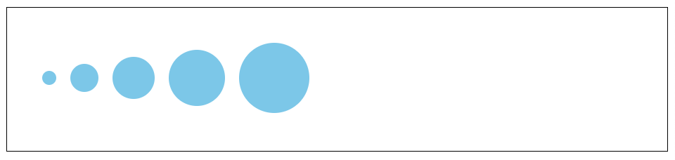
On this code snippet above:

• The selectAll() technique is used to create a collection of present circle parts in an SVG.
• The knowledge() technique binds the info array to this choice.
• The be a part of() technique is then used to deal with the brand new knowledge factors by appending new circle parts for every knowledge level.
• We additionally modify every circle attribute based mostly on the info (d) utilizing the attr() technique.

Loading knowledge in D3.js

D3.js gives varied data-loading strategies to accommodate totally different knowledge codecs. As an example, the d3.csv() technique masses knowledge from a comma-separated values (CSV) file. Equally, there are strategies like d3.tsv() for tab-separated values and d3.textual content() for plain textual content recordsdata. The flexibility of those strategies permits you to combine totally different knowledge sources into your visualizations seamlessly. You possibly can confer with the D3 documentation to view all of the file codecs you possibly can parse utilizing D3.js.

Let’s take a look at a easy instance utilizing d3.json() to load JSON knowledge right into a desk:

import { useEffect } from "react";
import * as d3 from "d3";

perform App() {
  useEffect(() => {
    
    d3.json(
      "https://js.devexpress.com/React/Demos/WidgetsGallery/JSDemos/knowledge/simpleJSON.json",
    ).then((knowledge) => {
      
      const desk = d3.choose("#salesTable");

      
      desk
        .append("thead")
        .append("tr")
        .selectAll("th")
        .knowledge(Object.keys(knowledge[0])) 
        .be a part of("th")
        .textual content((d) => d);

      
      desk
        .append("tbody")
        .selectAll("tr")
        .knowledge(knowledge)
        .be a part of("tr")
        .selectAll("td")
        .knowledge((d) => Object.values(d))
        .be a part of("td")
        .textual content((d) => d);
    });
  }, []);

  return <desk id="salesTable"></desk>;
}

export default App;

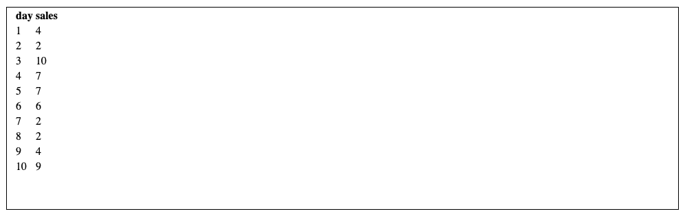
This instance makes use of the d3.json() technique to load knowledge from a JSON file asynchronously. As soon as the info is loaded, we leverage it to create our desk by making use of the choice, modification, and knowledge be a part of strategies we’ve explored earlier on this information.

Let React take the lead in rendering

In our earlier examples, we’ve been utilizing D3 (be a part of()) so as to add parts to the DOM on mount, however this isn’t the perfect method. React is a rendering library optimized for net functions, and immediately manipulating the DOM utilizing D3 as an alternative of JSX can work in opposition to these optimizations.

One other benefit of utilizing React for rendering is its declarative nature. Not like the crucial method with D3, the place you specify how to attract every factor, React’s JSX permits you to describe what is being drawn. This paradigm shift simplifies code comprehension and upkeep, which makes the event course of extra intuitive and collaborative.

With these benefits in thoughts, let’s modify our earlier code instance to make use of React for rendering our parts:

import { useEffect, useState } from "react";
import * as d3 from "d3";

perform App() {
  const [data, setData] = useState([]);
  const [loading, setLoading] = useState(true);

  useEffect(() => {
    const fetchData = async () => {
      setLoading(true);
      
      await d3
        .json(
          "https://js.devexpress.com/React/Demos/WidgetsGallery/JSDemos/knowledge/simpleJSON.json",
        )
        .then((knowledge) => {
          setData(knowledge);
        });
      setLoading(false);
    };
    fetchData();
  }, []);

  if (loading) return <p>Loading...</p>;

  return (
    <desk id="salesTable">
      <thead>
        <tr>
          {Object.keys(knowledge[0]).map((d) => (
            <th key={d}>{d}</th>
          ))}
        </tr>
      </thead>
      <tbody>
        {knowledge.map((d) => (
          <tr key={d.day}>
            <td>{d.day}</td>
            <td>{d.gross sales}</td>
          </tr>
        ))}
      </tbody>
    </desk>
  );
}

export default App;

Within the snippet above:

• We added a loading and knowledge state to trace the request’s standing and save the info.
• We use D3 to fetch the JSON knowledge inside a useEffect after which use JSX to render the desk, resulting in a lot cleaner and extra environment friendly code.

Creating Fundamental Knowledge Visualizations

Making a Bar Chart: Scales and Axes in D3

Now that we’ve established some groundwork for integrating D3.js with React, let’s dive into creating the primary visualization for our dashboard — a traditional bar chart. This visualization can even function a strong basis to know vital ideas like scales and axes in D3.

First, let’s learn to draw bars in a bar chart. Create a BarChart element in your parts listing and add the next code:

const barWidth = 60;

const BarChart = ({ width, peak, knowledge }) => {
  return (
    <div className="container">
      <svg className="viz" width={width} peak={peak} viewBox={`0 0 ${width} ${peak}`}>
        <g className="bars">
          {knowledge.map((d, i) => (
            <rect
              key={i}
              width={barWidth}
              peak={d}
              x={i * (barWidth + 5)}
              y={peak - d}
              fill="#6baed6"
            />
          ))}
        </g>
      </svg>
    </div>
  );
};

export default BarChart;

On this code:

• The knowledge array accommodates values representing the peak of every bar within the chart.
• The peak and width props signify the size of the svg container whereas the barWidth defines the width of every bar within the chart.
• Inside the <g> factor, we map by means of the knowledge array, create a <rect> factor for every bar within the chart, after which appropriately set their width, peak, and viewBox attributes.
• We use i * (barWidth + 5) for every x coordinate as a result of we wish the bars to have 5px area between one another.
• For the y coordinate, we use peak - d to make the bars go from backside to prime and look pure.
• The fill=" #6baed6" attribute units the fill coloration of every bar to a shade of blue.

Notice: we usually use <svg> parts for visualizations as a result of they’re scalable (you possibly can scale them to any dimension with out dropping high quality) and appropriate for representing varied shapes important for creating numerous charts.

Subsequent, let’s render our bar chart within the App element:

import BarChart from "./parts/BarChart";

const knowledge = [130, 200, 170, 140, 130, 250, 160];

perform App() {
  return <BarChart width={450} peak={300} knowledge={knowledge} />;
}

export default App;

And with that, we now have some bars in our bar chart utilizing dummy knowledge.

Subsequent, we have to find out about scales. Scales in D3.js are capabilities that enable you to map your knowledge area (the vary of your knowledge values) to a visible vary (the dimensions of your chart). They make your visualizations look exact by precisely portraying your knowledge on the canvas.

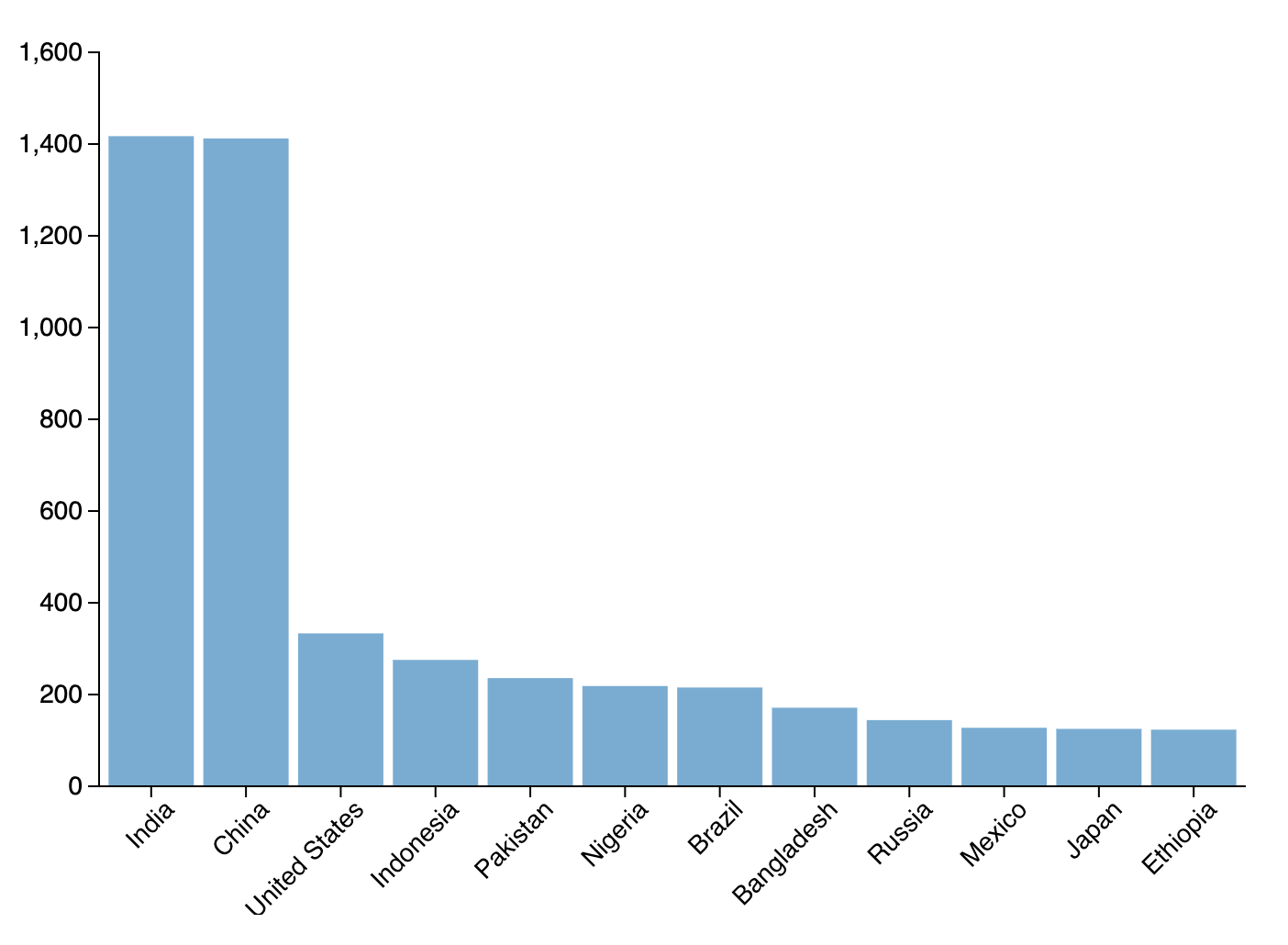
For instance, let’s check out the info we’ll be utilizing within the bar chart for our dashboard:

const knowledge = [
  { country: "India", population: 1_417_173_173 },
  { country: "China", population: 1_412_175_000 },
  { country: "United States", population: 333_287_557 },
  ...
];

The knowledge above represents the twelve most populous nations on this planet. With out utilizing scales, you may end up coping with the inhabitants knowledge utilizing pixel (px) values, that are impractical to deal with manually.

Let’s discover how utilizing scales simplifies this course of. Navigate to the App element and add the next code:

import BarChart from "./parts/BarChart";

const knowledge = [
  { country: "India", population: 1_417_173_173 },
  { country: "China", population: 1_412_175_000 },
  { country: "United States", population: 333_287_557 },
  { country: "Indonesia", population: 275_501_339 },
  { country: "Pakistan", population: 235_824_862 },
  { country: "Nigeria", population: 218_541_212 },
  { country: "Brazil", population: 215_313_498 },
  { country: "Bangladesh", population: 171_186_372 },
  { country: "Russia", population: 144_236_933 },
  { country: "Mexico", population: 127_504_125 },
  { country: "Japan", population: 125_124_989 },
  { country: "Ethiopia", population: 123_379_924 },
];

perform App() {
  return <BarChart width={700} peak={500} knowledge={knowledge} />;
}

export default App;

Within the snippet above, we’ve up to date the knowledge array to our inhabitants knowledge and elevated the width and peak of the bar chart to account for the elevated knowledge factors.

Subsequent, let’s replace our BarChart element to have scales:

import * as d3 from "d3";

const BarChart = ({ width, peak, knowledge }) => {
  
  const xScale = d3
    .scaleBand()
    .area(knowledge.map((d) => d.nation))
    .vary([0, width])
    .padding(0.1);

  
  const yScale = d3
    .scaleLinear()
    .area([0, d3.max(data, (d) => d.population)])
    .good()
    .vary([height, 0]);

  return (
    <div className="container">
      <svg width={width} peak={peak} className="viz" viewBox={`0 0 ${width} ${peak}`}>
        <g className="bars">
          {knowledge.map((d) => (
            <rect
              key={d.nation}
              x={xScale(d.nation)}
              y={yScale(d.inhabitants)}
              peak={peak - yScale(d.inhabitants)}
              width={xScale.bandwidth()}
              fill="#6baed6"
            />
          ))}
        </g>
      </svg>
    </div>
  );
};

export default BarChart;

Let’s clarify what’s new right here:

• xScale:

  • This makes use of D3’s scaleBand() for a band scale on the horizontal axis.
  • The area is about to the distinctive nation names within the knowledge for every band.
  • The vary is from 0 to the overall width of the <svg> container.
  • The padding introduces area between the bands.

• yScale:

  • This makes use of D3’s scaleLinear() for a linear scale on the vertical axis.
  • The area is about from 0 to the utmost inhabitants worth within the knowledge.
  • The good() technique adjusts the dimensions to incorporate good, spherical values.
  • The vary is from the overall peak of the <svg> container to 0 (reversed to match <svg> coordinates).

• We set the x and y coordinates of every <rect> created based on their respective scales (x={xScale(d.nation)} and y={yScale(d.inhabitants)}).

• We set the width of every <rect> utilizing xScale.bandwidth() so D3 sizes them relative to the width of our <svg>.

• Lastly, we set the peak of every <rect> to the <svg> peak after which subtract the peak generated by the yScale(d.inhabitants), ensuring every <rect> is represented accurately.

Whereas our scaled bar chart can now precisely signify knowledge, it’s lacking some context. A consumer viewing this wouldn’t know what every bar represents or what worth the peak interprets to. That is the place axes come into play. Axes in D3 present reference factors and labels, aiding viewers in understanding the dimensions of the visualization.

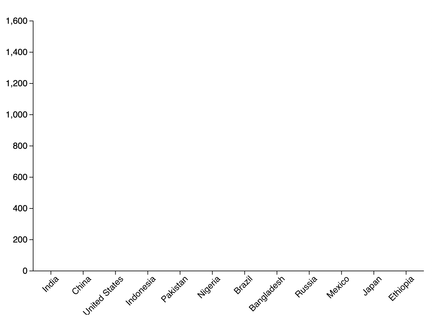
For our bar chart, we wish two axes:

• One on the backside of our chart that marks the identify of every nation on its respective bar.
• One on the left facet of our chart gives reference factors for the inhabitants in hundreds of thousands.

So as to add these axes correctly, we additionally want so as to add margins to our <svg> container to account for the axes. Let’s replace our BarChart element to implement these additions:

import { useEffect } from "react";
import * as d3 from "d3";

const marginTop = 30;
const marginBottom = 70;
const marginLeft = 50;
const marginRight = 25;
const oneMillion = 1_000_000;

const BarChart = ({ width, peak, knowledge }) => {
  const chartBottomY = peak - marginBottom;

  
  const xScale = d3
    .scaleBand()
    .area(knowledge.map((d) => d.nation))
    .vary([marginLeft, width - marginRight])
    .padding(0.1);

  const xAxis = d3.axisBottom(xScale).tickSizeOuter(0);

  
  const yScale = d3
    .scaleLinear()
    .area([0, d3.max(data, (d) => d.population / oneMillion)])
    .good()
    .vary([chartBottomY, marginTop]);

  const yAxis = d3.axisLeft(yScale);

  useEffect(() => {
    d3.choose(".x-axis")
      .name(xAxis)
      .selectAll("textual content")
      .attr("font-size", "14px")
      
      .attr("remodel", "rotate(-45)")
      .attr("text-anchor", "finish");
    d3.choose(".y-axis")
      .name(yAxis)
      .selectAll("textual content")
      .attr("font-size", "14px");
  }, [xAxis, yAxis]);

  return (
    <div className="container">
      <svg
        width={width}
        peak={peak}
        viewBox={`0 0 ${width} ${peak}`}
        className="viz"
      >
        <g className="bars">
          {knowledge.map((d) => (
            <rect
              key={d.nation}
              x={xScale(d.nation)}
              y={yScale(d.inhabitants / oneMillion)}
              peak={chartBottomY - yScale(d.inhabitants / oneMillion)}
              width={xScale.bandwidth()}
              fill="#6baed6"
            />
          ))}
        </g>
        <g className="x-axis" remodel={`translate(0,${chartBottomY})`}></g>
        <g className="y-axis" remodel={`translate(${marginLeft},0)`}></g>
      </svg>
    </div>
  );
};

export default BarChart;

Let’s break this down little by little:

• Part constants:

  • marginTop, marginBottom, marginLeft, and marginRight are the constants that outline the margins across the SVG chart space.
  • oneMillion is a scaling issue used to normalize inhabitants values for higher illustration on the y-axis of the bar chart. For instance, if a rustic has a inhabitants of three,000,000, the scaled-down worth can be 3. This scaling makes the axis labels and tick marks extra manageable for the viewer.
  • chartBottomY is calculated as peak - marginBottom, representing the y-coordinate of the underside fringe of the chart space.

• Horizontal (X) scale and axis:

  • xScale.vary() adjusts for the left and proper margins.
  • xAxis is an axis generator for the x-axis, configured to make use of xScale. tickSizeOuter(0) removes the tick mark on the outer fringe of the x-axis.

• Vertical (Y) scale and axis:

  • yScale.vary() adjusts for the highest and backside margins.
  • yAxis is an axis generator for the y-axis, configured to make use of yScale.

• useEffect for axis rendering:

  • The useEffect hook renders the x-axis and y-axis when the element mounts or when the xAxis or yAxis configurations change.
  • The selectAll("textual content") half selects all textual content parts inside the axis for additional styling.

• SVG teams for axes:

  • Two <g> (group) parts with class names "x-axis" and "y-axis" are appended to the SVG. We use these teams to render the x-axis and y-axis, respectively.
  • We use the remodel attribute to place the teams based mostly on the margins.

With these margin calculations and axis setups in place, our bar chart is way more organized and readable.

To make our bar chart much more readable, let’s add labels to every bar in our chart to signify their actual inhabitants:

...
<g className="bars">
    ...
</g>
<g className="labels">
  {knowledge.map((d) => (
      <textual content
          key={d.nation}
          x={xScale(d.nation) + xScale.bandwidth() / 2}
          y={yScale(d.inhabitants / oneMillion) - 5}
          textAnchor="center"
          fontSize={14}
        >
          {Quantity((d.inhabitants / oneMillion).toFixed(1)).toLocaleString()}
      </textual content>
  ))}
</g>
<g
  className="x-axis"
  ...
></g>
...

And there you could have it! With the scales, axes, and labels, our bar chart now precisely represents the info and gives beneficial context.

Making a pie chart

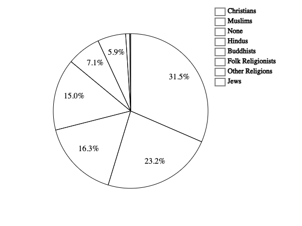
The following element we’ll construct for our dashboard is a pie chart. In D3.js, making a pie chart entails utilizing the pie() technique to generate angles for the info and the arc() technique to outline the form of every slice. We’ll additionally append a legend to the proper facet of the pie chart to hyperlink every arc’s coloration with a label.

The pie chart can be visualizing the world inhabitants by faith utilizing this knowledge:

const pieChartData = [
  { name: "Christians", value: 2_173_180_000 },
  { name: "Muslims", value: 1_598_510_000 },
  ...
];

Within the parts listing, create a PieChart element and add the next code:

import * as d3 from "d3";

const offsetX = 70;

const PieChart = ({ width, peak, knowledge }) => {
  
  const totalValue = knowledge.cut back((sum, faith) => sum + faith.worth, 0);

  
  let percentageData = {};
  knowledge.forEach((faith) => {
    percentageData[religion.name] = (
      (faith.worth / totalValue) *
      100
    ).toFixed(1);
  });

  
  const coloration = d3
    .scaleOrdinal(d3.schemeTableau10)
    .area(knowledge.map((d) => d.identify));

  
  const pie = d3
    .pie()
    .worth((d) => d.worth);

  const outerRadius = Math.min(width - 2, peak - 2) / 2 - offsetX;

  const arc = d3.arc().innerRadius(0).outerRadius(outerRadius);

  
  const labelRadius = arc.outerRadius()() * 0.75;
  const arcLabel = d3.arc().innerRadius(labelRadius).outerRadius(labelRadius);

  const arcs = pie(knowledge);

  return (
    <div className="container">
      <svg
        width={width}
        peak={peak}
        viewBox={`${-width / 2 + offsetX} ${-peak / 2} ${width} ${peak}`}
        className="viz"
      >
        {arcs.map((d, i) => (
          <g key={d.knowledge.identify} stroke="white">
            <path d={arc(d)} fill={coloration(knowledge[i].identify)} />
            <textual content
              x={arcLabel.centroid(d)[0]}
              y={arcLabel.centroid(d)[1]}
              textAnchor="center"
              stroke="none"
              fontSize={16}
              strokeWidth={0}
              fill="white"
            >
              {percentageData[d.data.name] > 5
                ? `${percentageData[d.data.name]}%`
                : ""}
            </textual content>
          </g>
        ))}

        {}
        <g>
          {knowledge.map((d, i) => {
            const x = outerRadius + 14;
            const y = -peak / 2 + i * 20 + 20;

            return (
              <g key={d.identify}>
                <rect x={x} y={y} width={20} peak={15} fill={coloration(d.identify)} />
                <textual content
                  x={x}
                  y={y}
                  dx={25}
                  fontSize={14}
                  alignmentBaseline="hanging"
                >
                  {d.identify}
                </textual content>
              </g>
            );
          })}
        </g>
      </svg>
    </div>
  );
};

export default PieChart;

Let’s analyze the code:

• Whole worth calculation:

  • The totalValue is calculated by summing up every knowledge level’s worth property.

• Proportion knowledge calculation:

  • The share contribution to the overall worth is calculated and formatted for every knowledge level. We then retailer the leads to the percentageData object.

• Coloration scale creation:

• Pie structure and arc generator setup:

  • The pie structure is created utilizing d3.pie().worth((d) => d.worth). The worth((d) => d.worth) snippet determines how the pie will extract the info values for every slice.
  • An outer radius (outerRadius) is calculated based mostly on the minimal worth between the width and peak, after which an offset (offsetX) is added to the end result.
  • An arc generator (arc) is created with an inside radius of 0 and the calculated outer radius.
  • A separate arc generator (arcLabel) is created for displaying labels. It has a particular inside and outer radius.

• Pie knowledge technology:

  • The pie structure is utilized to the info (pie(knowledge)), producing an array of arcs.

• SVG rendering:

  • The <svg> container has specified width, peak, and viewBox attributes. The viewBox is adjusted to incorporate an offset (offsetX) for higher centering.
  • For every arc within the arcs array, a <path> factor is created, representing a pie slice. We set the fill attribute utilizing the colour scale.
  • Textual content labels are added to every pie slice. The share worth is displayed if the proportion is bigger than 5%.

• Legend rendering:

  • A legend entry is created for every knowledge level with a coloured rectangle and the faith identify. We place the legend to the proper of the pie chart.

Subsequent, let’s add our knowledge and pie chart to the App.jsx file:

import PieChart from "./parts/PieChart";

const pieChartData = [
  { name: "Christians", value: 2_173_180_000 },
  { name: "Muslims", value: 1_598_510_000 },
  { name: "None", value: 1_126_500_000 },
  { name: "Hindus", value: 1_033_080_000 },
  { name: "Buddhists", value: 487_540_000 },
  { name: "Folk Religionists", value: 405_120_000 },
  { name: "Other Religions", value: 58_110_000 },
  { name: "Jews", value: 13_850_000 },
];

perform App() {
  return <PieChart width={750} peak={450} knowledge={pieChartData} />;
}

export default App;

And right here’s our preview:

Making a map

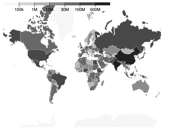
The final element we’ll create for our dashboard is a choropleth map, which we’ll use to visualise the world inhabitants by nation. This choropleth map will visually signify the inhabitants distribution, coloring every area based on a numeric variable.

To assemble a choropleth map, we first want the 2D coordinates outlining the boundaries of every area — in our case, the nations. This info is usually saved in a GeoJSON format. GeoJSON is a typical file format utilized in geographic info programs, representing geographical options and their attributes:

{
  "sort": "FeatureCollection",
  "options": [
    {
      "type": "Feature",
      "id": "AFG",
      "properties": { "name": "Afghanistan" },
      "geometry": {
        "type": "Polygon",
        "coordinates": []
      }
    },
    
  ]
}

We’ll additionally want the inhabitants knowledge that gives a inhabitants worth for every nation within the GeoJSON file. Let’s fetch these assets in our App element:

import { useEffect, useState } from "react";
import * as d3 from "d3";

const pieChartData = [
  ...
];

perform App() {
  const [worldPopulation, setWorldPopulation] = useState(null);
  const [topography, setTopography] = useState(null);
  const [loading, setLoading] = useState(true);

  useEffect(() => {
    const getData = async () => {
      setLoading(true);

      let populationData = {};
      await Promise.all([
        d3.json(
          "https://res.cloudinary.com/tropicolx/raw/upload/v1/Building%20Interactive%20Data%20Visualizations%20with%20D3.js%20and%20React/world.geojson"
        ),
        d3.csv(
          "https://res.cloudinary.com/tropicolx/raw/upload/v1/Building%20Interactive%20Data%20Visualizations%20with%20D3.js%20and%20React/world_population.csv",
          (d) => {
            populationData = {
              ...populationData,
              [d.code]: +d.inhabitants,
            };
          }
        ),
      ]).then((fetchedData) => {
        const topographyData = fetchedData[0];
        setWorldPopulation(populationData);
        setTopography(topographyData);
      });

      setLoading(false);
    };

    getData();
  }, []);

  if (loading) return <div>Loading...</div>;

  return (
    <WorldMap width={550} peak={450} knowledge={{ worldPopulation, topography }} />
  );
}

export default App;

In our up to date App element:

• The useEffect hook is employed to fetch knowledge from two totally different sources: a GeoJSON file and a CSV file.
• The GeoJSON knowledge represents the world topography, whereas the CSV knowledge accommodates inhabitants info by nation code.
• The fetched knowledge is saved in state variables (worldPopulation and topography), which we move into the WorldMap element as a prop.

Subsequent, let’s create a Legend element for our map to render a coloration scale legend based mostly on the supplied coloration scale:

import { useEffect, useRef } from "react";
import * as d3 from "d3";

const Legend = ({
  coloration,
  tickSize = 6,
  width = 320,
  peak = 44 + tickSize,
  marginTop = 18,
  marginRight = 0,
  marginBottom = 16 + tickSize,
  marginLeft = 0,
  ticks = width / 64,
  tickFormat,
  tickValues,
} = {}) => {
  const svgRef = useRef(null);

  
  const thresholds = coloration.thresholds
    ? coloration.thresholds() 
    : coloration.quantiles
      ? coloration.quantiles() 
      : coloration.area(); 

  const thresholdFormat =
    tickFormat === undefined
      ? (d) => d
      : typeof tickFormat === "string"
        ? d3.format(tickFormat)
        : tickFormat;

  const x = d3
    .scaleLinear()
    .area([-1, color.range().length - 1])
    .rangeRound([marginLeft, width - marginRight]);

  tickValues = d3.vary(thresholds.size);
  tickFormat = (i) => thresholdFormat(thresholds[i], i);

  useEffect(() => {
    let tickAdjust = (g) =>
      g.selectAll(".tick line").attr("y1", marginTop + marginBottom - peak);

    d3.choose(".ticks")
      .name(
        d3
          .axisBottom(x)
          .ticks(ticks, typeof tickFormat === "string" ? tickFormat : undefined)
          .tickFormat(typeof tickFormat === "perform" ? tickFormat : undefined)
          .tickSize(tickSize)
          .tickValues(tickValues),
      )
      .name(tickAdjust)
      .name((g) => g.choose(".area").take away())
      .name((g) => g.selectAll("textual content").attr("font-size", "14px"));
  }, []);

  return (
    <svg ref={svgRef} width={width} peak={peak}>
      <g>
        {coloration.vary().map((d, i) => (
          <rect
            key={d}
            x={x(i - 1)}
            y={marginTop}
            width={x(i) - x(i - 1)}
            peak={peak - marginTop - marginBottom}
            fill={d}
          />
        ))}
      </g>
      <g
        className="ticks"
        remodel={`translate(0, ${peak - marginBottom})`}
      ></g>
    </svg>
  );
};

export default Legend;

Lots is happening right here, however let’s simplify it by breaking down the important parts:

• The thresholds variable extracts threshold values from the colour scale.
• We place the tick marks on the legend utilizing the x linear scale.
• The useEffect hook units up the axis utilizing d3.axisBottom(x) and adjusts tick positions. It additionally removes the area line and units the font dimension for higher visibility.
• Coloured rectangles are rendered based mostly on the colour scale’s vary, representing totally different colours within the legend.
• The returned JSX renders an SVG factor containing coloured rectangles and an axis for reference.

Now that we’ve arrange our map’s knowledge and legend, let’s delve into our WorldMap element:

import * as d3 from "d3";

import Legend from "./Legend";

const WorldMap = ({ width, peak, knowledge }) => {
  const worldPopulation = knowledge.worldPopulation;
  const topography = knowledge.topography;

  
  const path = d3.geoPath();
  const projection = d3
    .geoMercator()
    .scale(85)
    .heart([0, 30])
    .translate([width / 2, height / 2]);

  const pathGenerator = path.projection(projection);

  
  const colorScale = d3
    .scaleThreshold()
    .area([100000, 1000000, 10000000, 30000000, 100000000, 500000000])
    .vary(d3.schemeBlues[7]);

  return (
    <div className="container">
      <svg
        className="viz"
        width={width}
        peak={peak}
        viewBox={`0 0 ${width} ${peak}`}
      >
        <g className="topography">
          {topography.options.map((d) => (
            <path
              key={d.id}
              d={pathGenerator(d)}
              fill=
              stroke="#FFFFFF"
              strokeWidth={0.3}
            />
          ))}
        </g>

        {}
        <g className="legend" remodel="translate(10,10)">
          <Legend
            coloration={colorScale}
            width={peak / 1.25}
            tickFormat={d3.format("~s")}
          />
        </g>
      </svg>
    </div>
  );
};

export default WorldMap;

Let’s break down every part of the code:

• Projection and path generator:

  • We outline a projection utilizing d3.geoMercator() to rework 3D GeoJSON coordinates right into a 2D area.
  • We use scale() technique on the projection to find out the zoom stage of the map.
  • We use the heart() technique to set the middle of the map in geographical coordinates.
  • The translate() technique shifts the projection’s heart to a particular level on the SVG canvas. We use [width / 2, height / 2] because the coordinates to put the middle of the map on the heart of the SVG canvas
  • The pathGenerator makes use of this projection to generate paths for every area.

• Coloration scale:

  • A colorScale is created utilizing d3.scaleThreshold() to map the inhabitants values to colours. It’s a sequential coloration scheme from mild to darkish blue (d3.schemeBlues[7]) on this case.

• Rendering topography options:

  • We map by means of GeoJSON options, producing a <path> factor for every nation. The colour scale determines the fill attribute based mostly on the corresponding world inhabitants knowledge.

• Legend element:

  • We embrace the legend element to supply a visible information to interpret the colour scale.

The demo beneath exhibits the output.

Enhancing Interactivity

We’ve constructed out all of the visualizations for our dashboard, however they nonetheless lack one thing essential: interactivity. Including interactive parts to your visualizations permits customers to discover the info dynamically, making it simpler to realize insights by interacting immediately with the visualization. Let’s discover methods to implement interactive options like tooltips, zooming, and panning utilizing D3.js.

Implementing tooltips

Tooltips are a easy but efficient means to supply further info when customers hover over knowledge factors. Let’s begin by enhancing our pie chart with tooltips:

import { useState } from "react";
...

const PieChart = ({ width, peak, knowledge }) => {
  const [tooltipVisible, setTooltipVisible] = useState(false);
  const [tooltipData, setTooltipData] = useState({
    ...knowledge[0],
    x: 0,
    y: 0,
  });

  ...

  return (
    <div className="container">
      <svg
        ...
      >
        {arcs.map((d, i) => (
          <g
            ...
            onMouseOver={() => setTooltipVisible(true)}
            onMouseLeave={() => setTooltipVisible(false)}
            onMouseMove={() => {
              setTooltipData({
                ...knowledge[i],
                x: arcLabel.centroid(d)[0],
                y: arcLabel.centroid(d)[1],
              });
            }}
          >
            ...
          </g>
        ))}

        {}
        <g>
          ...
        </g>

        {}
        <g
          onMouseEnter={() => setTooltipVisible(true)}
          onMouseLeave={() => setTooltipVisible(false)}
          className={`tooltip ${tooltipVisible ? "seen" : ""}`}
        >
          <rect
            width={200}
            peak={60}
            x={tooltipData.x - 10}
            y={tooltipData.y + 10}
            stroke="#cccccc"
            strokeWidth="1"
            fill="#ffffff"
          ></rect>
          <g>
            <textual content
              textAnchor="begin"
              x={tooltipData.x}
              y={tooltipData.y + 35}
              fontSize={16}
            >
              {tooltipData.identify}
            </textual content>
          </g>
          <g>
            <textual content
              textAnchor="begin"
              x={tooltipData.x}
              y={tooltipData.y + 55}
              fontSize={16}
              fontWeight="daring"
            >
              {tooltipData.worth.toLocaleString()}
              {` (${percentageData[tooltipData.name]}%)`}
            </textual content>
          </g>
        </g>
      </svg>
    </div>
  );
};

export default PieChart;

Let’s clarify what’s happening right here:

• State for tooltip visibility and knowledge:

  • Two items of state are launched utilizing the useState hook: tooltipVisible to trace whether or not the tooltip is seen, and tooltipData to retailer the info for the tooltip.

• Mouse occasions in pie slices:

  • For every pie slice (<g> factor representing a slice), we add the onMouseOver, onMouseLeave, and onMouseMove occasion handlers.
  • onMouseOver and onMouseLeave units tooltipVisible to true and false, respectively.
  • onMouseMove updates the tooltipData with the corresponding knowledge and the centroid coordinates for the tooltip place.

• Tooltip rendering:

  • A separate <g> factor is added to the SVG to signify the tooltip.
  • The onMouseEnter and onMouseLeave occasion handlers are additionally hooked up to this tooltip group to regulate its visibility.
  • The CSS class seen is conditionally utilized to the tooltip group based mostly on the tooltipVisible state to regulate the tooltip’s visibility.
  • Inside the tooltip group, we add a <rect> factor to create a background for the tooltip, and we use two <textual content> parts to show the faith’s identify and worth.

• Tooltip positioning:

  • The x and y attributes of the <rect> factor are set based mostly on the tooltipData.x and tooltipData.y values. This technique ensures that the tooltip’s place is on the centroid of the corresponding pie slice.
  • The textual content parts contained in the tooltip are positioned relative to the tooltipData.x and tooltipData.y values.

• Conditional show of tooltip content material:

  • The tooltip’s content material is dynamically set based mostly on the tooltipData, displaying the faith identify, worth (formatted with toLocaleString()), and the proportion.

• CSS styling for tooltip visibility:

  • The CSS class seen is conditionally utilized to the tooltip group based mostly on the tooltipVisible state. This class controls the visibility of the tooltip.

Subsequent, let’s head to the index.css file and add the next CSS code:

* {
  margin: 0;
  padding: 0;
  font-family: "Roboto", sans-serif;
  box-sizing: border-box;
}

.container {
  place: relative;
  overflow: hidden;
}

.tooltip {
  show: none;
  background: white;
  border: strong;
  border-width: 2px;
  border-radius: 5px;
  padding: 5px;
  place: absolute;
}

.tooltip.seen {
  show: block;
}

Within the snippet above, we’ve outlined the container properties for the chart and styled the tooltip that seems when interacting with the pie chart. Moreover, we’ve added the seen class to dynamically management the visibility of the tooltip based mostly on its state.

The demo beneath exhibits the output.

With all this in place, when customers hover over every slice within the chart, they’ll obtain on the spot insights into the corresponding knowledge factors.

Our WorldMap visualization additionally wants tooltips to point out extra particulars about every nation when interacting with it. Let’s head over to the WorldMap element and add the next code:

import { useRef, useState } from "react";
import * as d3 from "d3";

import Legend from "./Legend";

const WorldMap = ({ width, peak, knowledge }) => {
    ...

    const chartRef = useRef(null);
    const [tooltipVisible, setTooltipVisible] = useState(false);
    const [tooltipData, setTooltipData] = useState({
        identify: "",
        inhabitants: "",
        x: 0,
        y: 0,
    });

    ...

    return (
        <div className="container">
            <svg
                ref={chartRef}
                ...
            >
                <g className="topography">
                    {topography.options.map((d) => (
                        <path
                            ...
                            onMouseEnter={() => {
                                setTooltipVisible(true);
                            }}
                            onMouseLeave={() => {
                                setTooltipVisible(false);
                            }}
                            onMouseMove={(occasion) => {
                                const inhabitants = (
                                    worldPopulation[d.id] || "N/A"
                                ).toLocaleString();

                                
                                const [x, y] = d3.pointer(
                                    occasion,
                                    chartRef.present
                                );

                                setTooltipData({
                                    identify: d.properties.identify,
                                    inhabitants,
                                    left: x - 30,
                                    prime: y - 80,
                                });
                            }}
                        />
                    ))}
                </g>

                {}
                <g className="legend" remodel="translate(10,10)">
                    ...
                </g>
            </svg>

            {}
            {tooltipData && (
                <div
                    className={`tooltip ${tooltipVisible ? "seen" : ""}`}
                    fashion={{
                        left: tooltipData.left,
                        prime: tooltipData.prime,
                    }}
                >
                    {tooltipData.identify}
                    <br />
                    {tooltipData.inhabitants}
                </div>
            )}
        </div>
    );
};

export default WorldMap;

This implementation is similar to our earlier instance, however with a couple of distinctions:

• We use d3.pointer() to place the tooltip based mostly on the present mouse or contact occasion coordinates relative to the <svg> factor.
• We use a <div> factor exterior the <svg> for the tooltip as an alternative of a <g> factor inside the <svg>.

Implementing zooming and panning

Zooming and panning add a layer of sophistication to our visualizations, enabling customers to simply discover massive datasets. Let’s improve our map with zooming and panning capabilities:

import { useEffect, useRef, useState } from "react";
...

const WorldMap = ({ width, peak, knowledge }) => {
    ...

    const zoom = d3
        .zoom()
        .scaleExtent([1, 8])
        .on("zoom", (occasion) => {
            const { remodel } = occasion;
            setMapStyle({
                remodel: `translate(${remodel.x}px, ${remodel.y}px) scale(${remodel.ok})`,
                strokeWidth: 1 / remodel.ok,
            });
        });

    perform reset() {
        const svg = d3.choose(chartRef.present);
        svg.transition()
            .length(750)
            .name(
                zoom.remodel,
                d3.zoomIdentity,
                d3.zoomTransform(svg.node()).invert([width / 2, height / 2])
            );
    }

    useEffect(() => {
        const svg = d3.choose(chartRef.present);
        svg.name(zoom);
    }, [zoom]);

    return (
        <div className="container">
            <svg
                ...
                onClick={() => reset()}
            >
                ...
            </svg>

            ...
        </div>
    );
};

export default WorldMap;

Let’s break down what’s happening right here:

With these additions, the WorldMap element now incorporates zooming and panning capabilities. Customers can interactively discover the choropleth map by zooming out and in and resetting the view. This characteristic enhances the consumer expertise and gives a extra detailed examination of the worldwide inhabitants distribution.

Actual-world Instance: World Inhabitants Dashboard

Constructing the dashboard

Constructing on our basis of interactive visualizations, let’s take the following step and create our full dashboard. Firstly, let’s put all of the items collectively in our App element:

import { useEffect, useState } from "react";
import * as d3 from "d3";

import BarChart from "./parts/BarChart";
import PieChart from "./parts/PieChart";
import WorldMap from "./parts/WorldMap";

const pieChartData = [
    { name: "Christians", value: 2_173_180_000 },
    { name: "Muslims", value: 1_598_510_000 },
    { name: "None", value: 1_126_500_000 },
    { name: "Hindus", value: 1_033_080_000 },
    { name: "Buddhists", value: 487_540_000 },
    { name: "Folk Religionists", value: 405_120_000 },
    { name: "Other Religions", value: 58_110_000 },
    { name: "Jews", value: 13_850_000 },
];

perform App() {
    ...
    const [barChartData, setBarChartData] = useState([]);
    const [loading, setLoading] = useState(true);

    useEffect(() => {
        const getData = async () => {
            ...
            await Promise.all([
                ...
            ]).then((fetchedData) => {
                const topographyData = fetchedData[0];
                const barChartData = topographyData.options
                    .map((d) => ( 0,
                    ))
                    .kind((a, b) => b.inhabitants - a.inhabitants)
                    .slice(0, 12);
                setBarChartData(barChartData);
                ...
            });
            ...
        };

        getData();
    }, []);

    if (loading) return <div>Loading...</div>;

    return (
        <div className="dashboard">
            <div className="wrapper">
                <h1>
                    <span className="skinny">World</span>
                    <span className="daring">Inhabitants</span> Insights 2022
                </h1>
                <essential className="essential">
                    <div className="grid">
                        <div className="card stat-card">
                            <h2>Whole Inhabitants</h2>
                            <span className="stat">7.95B</span>
                        </div>
                        <div className="card stat-card">
                            <h2>Male Inhabitants</h2>
                            <span className="stat">4B</span>
                        </div>
                        <div className="card stat-card">
                            <h2>Feminine Inhabitants</h2>
                            <span className="stat">3.95B</span>
                        </div>
                        <div className="card map-container">
                            <h2>World Inhabitants by Nation</h2>
                            <WorldMap
                                width={550}
                                peak={450}
                                knowledge={{ worldPopulation, topography }}
                            />
                        </div>
                        <div className="card pie-chart-container">
                            <h2>World Inhabitants by Faith</h2>
                            <PieChart
                                width={650}
                                peak={450}
                                knowledge={pieChartData}
                            />
                        </div>
                        <div className="card bar-chart-container">
                            <h2>High International locations by Inhabitants (in hundreds of thousands)</h2>
                            <BarChart
                                width={1248}
                                peak={500}
                                knowledge={barChartData}
                            />
                        </div>
                    </div>
                </essential>
            </div>
        </div>
    );
}

export default App;

In our up to date App element:

• We use the inhabitants knowledge derived for our WorldMap to generate our BarChart knowledge.
• The primary construction of the dashboard is outlined inside the return assertion.
• We added playing cards displaying the overall inhabitants, and the female and male populations.
• Containers for the world map, pie chart, and bar chart are arrange with corresponding titles.
• Every visualization element (WorldMap, PieChart, BarChart) receives the required knowledge and dimensions.

Subsequent, let’s fashion our dashboard. Within the index.css file add the next code:

...

physique {
  background-color: #eff2f7;
}

h1 {
  padding-top: 30px;
  padding-bottom: 40px;
  font-size: 1.2rem;
  font-weight: 200;
  text-transform: capitalize;
  coloration: #1ca4d9;
}

.skinny,
.daring {
  font-size: 2rem;
  text-transform: uppercase;
}

h1 .daring {
  font-weight: 700;
}

h2 {
  font-size: 1.5rem;
  font-weight: 500;
}

.viz {
  width: 100%;
  peak: auto;
}

.dashboard {
  padding-left: 1rem;
  padding-right: 1rem;
}

.wrapper {
  margin: 0 auto;
}

.essential {
  padding-bottom: 10rem;
}

.grid {
  show: grid;
  hole: 14px;
}

.map-container,
.pie-chart-container,
.bar-chart-container,
.card {
  show: flex;
  flex-direction: column;
  justify-content: space-between;
  hole: 10px;
  padding: 1rem;
  border-radius: 0.75rem;
  --tw-shadow: 0px 0px 0px 1px rgba(9, 9, 11, 0.07),
    0px 2px 2px 0px rgba(9, 9, 11, 0.05);
  --tw-shadow-colored: 0px 0px 0px 1px var(--tw-shadow-color),
    0px 2px 2px 0px var(--tw-shadow-color);
  box-shadow:
    0 0 #0000,
    0 0 #0000,
    var(--tw-shadow);
  background: white;
}

.stat-card {
  align-items: heart;
  justify-content: heart;
  peak: 200px;
}

.card .stat {
  font-size: 3rem;
  font-weight: 600;
  coloration: #1ca4d9;
}

.labels textual content {
  show: none;
}

@media (min-width: 1280px) {
  .grid {
    grid-template-columns: repeat(15, minmax(0, 1fr));
  }
}

@media (min-width: 1024px) {
  .wrapper {
    max-width: 80rem;
  }

  .container {
    overflow: seen;
  }

  .card {
    grid-column: span 5 / span 5;
  }

  .map-container {
    grid-column: span 7 / span 7;
  }

  .pie-chart-container {
    grid-column: span 8 / span 8;
  }

  .bar-chart-container {
    grid-column: span 15 / span 15;
  }
}

@media (min-width: 768px) {
  .labels textual content {
    show: block;
  }
}

This snippet types the structure and look of the dashboard and all its parts. The result’s proven beneath.

Making the visualizations responsive

Though we’ve arrange our dashboard’s structure and styling and made it responsive, the visualizations themselves usually are not responsive. In consequence, the visualizations shrink on smaller units, which makes the textual content and labels inside them arduous to learn. To deal with this concern, we will create a customized hook that ensures our visualizations reply seamlessly to the container dimension adjustments.

Create a hooks folder within the src listing and create a brand new useChartDimensions.jsx file. Add the next code:

import { useEffect, useRef, useState } from "react";

const combineChartDimensions = (dimensions) => {
  const parsedDimensions =  40,
    marginLeft: dimensions.marginLeft ;
  return {
    ...parsedDimensions,
    boundedHeight: Math.max(
      parsedDimensions.peak -
        parsedDimensions.marginTop -
        parsedDimensions.marginBottom,
      0
    ),
    boundedWidth: Math.max(
      parsedDimensions.width -
        parsedDimensions.marginLeft -
        parsedDimensions.marginRight,
      0
    ),
  };
};

const useChartDimensions = (passedSettings) => {
  const ref = useRef();
  const dimensions = combineChartDimensions(passedSettings);

  const [width, setWidth] = useState(0);
  const [height, setHeight] = useState(0);

  useEffect(() => {
    if (dimensions.width && dimensions.peak) return [ref, dimensions];

    const factor = ref.present;
    const resizeObserver = new ResizeObserver((entries) => {
      if (!Array.isArray(entries)) return;
      if (!entries.size) return;

      const entry = entries[0];

      if (width != entry.contentRect.width) setWidth(entry.contentRect.width);
      if (peak != entry.contentRect.peak)
        setHeight(entry.contentRect.peak);
    });
    resizeObserver.observe(factor);

    return () => resizeObserver.unobserve(factor);
  }, []);

  const newSettings = combineChartDimensions();

  return [ref, newSettings];
};

export default useChartDimensions;

Within the above snippet:

• We mix passedSettings with the default margin values and compute the bounded width and peak of the chart space.
• It then observes adjustments within the container’s dimensions utilizing the ResizeObserver.
• When a change happens, the hook updates the width and peak states accordingly.

Subsequent, let’s apply this hook to our visualizations. Let’s begin with our BarChart element:

...

import useChartDimensions from "../hooks/useChartDimensions";

...

const BarChart = ({ peak, knowledge }) => {
    const [ref, dms] = useChartDimensions({
        marginTop,
        marginBottom,
        marginLeft,
        marginRight,
    });
    const width = dms.width;
    ...

    return (
        <div
            ref={ref}
            fashion={{
                peak,
            }}
            className="container"
        >
            ...
        </div>
    );
};

export default BarChart;

After which the PieChart element:

...

import useChartDimensions from "../hooks/useChartDimensions";

...

const PieChart = ({ peak, knowledge }) => {
    const [ref, dms] = useChartDimensions({});
    const width = dms.width;
    ...

    return (
        <div
            ref={ref}
            fashion={{
                peak,
            }}
            className="container"
        >
            ...
        </div>
    );
};

export default PieChart;

And eventually, our WorldMap element:

...
import useChartDimensions from "../hooks/useChartDimensions";

const WorldMap = ({ peak, knowledge }) => {
    ...
    const [ref, dms] = useChartDimensions({});
    const width = dms.width;

    ...

    return (
        <div
            ref={ref}
            fashion={{
                peak,
            }}
            className="container"
        >
            ...
        </div>
    );
};

export default WorldMap;

Let’s take a look at some key issues happening in every of those parts:

• The useChartDimensions hook is utilized by calling it with both an empty object ({}) if no arguments are wanted or an object containing the element’s preliminary dimensions — for instance, its margins, like with the BarChart element.
• The hook returns a ref (ref) that must be hooked up to the factor whose dimensions you wish to observe, and an object (dms) containing the size info.
• The width variable is now not a prop however is assigned the worth of the width dimension obtained from the dms object. This worth dynamically updates because the container’s width adjustments.
• The ref is hooked up to the container div factor, permitting the useChartDimensions hook to look at adjustments in its dimensions. The peak is about as an inline fashion since we wish that to be static, after which the element’s rendering logic follows.

Since we’re indirectly setting the width of the parts anymore, we will take away their width props within the App element:

...
    <div className="card map-container">
        ...
        <WorldMap
            peak={450}
            knowledge={{ worldPopulation, topography }}
        />
    </div>
    <div className="card pie-chart-container">
        ...
        <PieChart
            peak={450}
            knowledge={pieChartData}
        />
    </div>
    <div className="card bar-chart-container">
        ...
        <BarChart
            peak={500}
            knowledge={barChartData}
        />
    </div>
...

And that’s it! We now have our totally responsive and interactive dashboard.

Greatest Practices and Optimization

Optimize efficiency

Think about the next ideas when making an attempt to optimize the efficiency of your visualizations:

• Memoization for dynamic updates. Memoization turns into helpful in case your dataset undergoes frequent updates or transformations. It prevents pointless recalculations and re-renders, enhancing the effectivity of your parts.
• Keep away from direct DOM manipulation. Let React deal with the DOM updates. Keep away from direct manipulation utilizing D3 which may intrude with React’s digital DOM.
• Knowledge aggregation. For datasets with a excessive quantity of factors, discover knowledge aggregation strategies to current significant summaries fairly than render each knowledge level.

Guarantee accessibility and responsiveness

Make your visualizations accessible to a various viewers and responsive throughout varied units:

• ARIA roles and labels. Incorporate ARIA (Accessible Wealthy Web Functions) roles and labels to reinforce accessibility. Present clear descriptions and labels for interactive parts.
• Responsive design. Guarantee your visualizations are responsive by adapting to totally different display sizes. Make the most of responsive design ideas, comparable to versatile layouts and media queries, to create an optimum consumer expertise on varied units.

Frequent pitfalls and challenges

• International state administration. Coping with knowledge updates and synchronization in D3 and React could be difficult. Make the most of a state administration device like Redux to centralize and synchronize knowledge adjustments throughout parts. This optimization will guarantee consistency and simplify the coordination of updates.
• Occasion bus sample. Implement an occasion bus sample to broadcast adjustments in a single visualization to others. This sample facilitates communication between parts, permitting for constant updates and lowering the complexity of managing shared state.
• Cross-browser compatibility. Check your visualizations throughout a number of browsers to make sure cross-browser compatibility. Whereas D3.js and React usually work effectively collectively, occasional discrepancies might come up. Thorough testing ensures a seamless expertise for customers on totally different browsers.

By adopting these finest practices and optimization methods, you possibly can make sure that your D3.js and React functions carry out effectively and stand the take a look at of time.

Conclusion

On this information, we supplied a complete walkthrough of integrating React and D3.js to create knowledge visualizations. We coated important ideas, from knowledge loading to factor manipulation, and demonstrated methods to construct varied visualizations, together with a bar chart, pie chart, and a choropleth map.

We additionally checked out methods to make our visualizations responsive utilizing a customized hook, which ensures adaptability throughout totally different display sizes. Lastly, we established a basis for constructing performant and interesting data-driven functions by adhering to finest practices and optimization methods.

When approached with precision, combining the declarative nature of React with the data-centric capabilities of D3.js yields highly effective and environment friendly knowledge visualizations that cater to each kind and performance.