Implementation, Evaluation & Adam Comparability

Introduction

Optimizing deep studying is a vital facet of coaching environment friendly and correct neural networks. Varied  optimization algorithms have been developed to enhance the convergence pace . One such Algorithm is Adahessian ,which is second-order optimization methodology recognized for its effectiveness in dealing with complicated landscapes. On this article we are going to delve into the working of the ada hessian optimizer, examine it with first-order differential optimizer, and discover the way it works and take steps to enhance convergence.

For a complete understanding, we are going to implement AdaHessian from scratch on a single neuron and visualize gradients in 3D plots. Our focus shall be on analyzing the outcomes of AdaHessian on this neuron and evaluating it with Adam, visualizing the comparisons in 3D plots.

Yow will discover the implementation particulars within the repository hyperlink.

Studying Goals

• Acquire insights into the variations between first-order and second-order optimization strategies, their strengths, and limitations in coaching neural networks.
• Acknowledge the challenges confronted by conventional optimization strategies, reminiscent of computational value, inaccurate Hessian approximation, and reminiscence overhead.
• Study AdaHessian as a second-order optimization algorithm that addresses these challenges by incorporating Hessian diagonal approximation, spatial averaging, and Hessian momentum.
• Perceive the elemental elements of AdaHessian, together with the Hessian diagonal, spatial averaging for curvature smoothing, and momentum methods for sooner convergence.
• Discover the sensible implementation of AdaHessian on a single neuron utilizing NumPy, specializing in visualizing gradients in 3D plots and evaluating its efficiency with AdamW.
• Develop a transparent understanding of how AdaHessian leverages Hessian info, spatial averaging, and momentum to enhance optimization stability and convergence pace.

 First-Order vs. Second-Order Optimization

• First-Order Optimization: First-order strategies, reminiscent of Gradient Descent (GD) and its variants like Adam and RMSProp, depend on gradient info (first derivatives) to replace mannequin parameters. They’re computationally inexpensive however could undergo from sluggish convergence in extremely non-linear and ill-conditioned optimization landscapes.

• Second-Order Optimization: Second-order strategies, like AdaHessian, consider not solely the gradients but in addition the curvature of the loss operate (second derivatives). This extra info can result in sooner convergence and higher dealing with of complicated optimization surfaces.

Lets perceive in regards to the  Second By-product Curvature info :

Second-Order Derivatives

• The second spinoff of a operate  f(x)  at a degree ( x ) provides us details about the curvature of the operate’s graph at that time.
•  If the second spinoff is constructive at a degree ( x ), it signifies that the operate is concave up (bowl-shaped), suggesting a minimal level. It is because the operate is curving upwards, like the underside of a bowl.
•  If the second spinoff is damaging at a degree ( x ), it signifies that the operate is concave down (bowl-shaped), suggesting a most level. It is because the operate is curving downwards, like the highest of a bowl.
•  A second spinoff of zero at a degree ( x ) suggests a attainable level of inflection. Some extent of inflection is the place the curvature adjustments path, reminiscent of transitioning from concave as much as concave down or vice versa. Nevertheless, additional investigation is required to substantiate the presence of a degree of inflection.

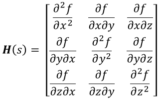
Hessian Matrix: For features of a number of variables, the Hessian matrix is a sq. matrix that incorporates all of the second-order partial derivatives of the operate. The diagonal parts of the Hessian matrix correspond to the second partial derivatives with respect to particular person variables, whereas the off-diagonal parts symbolize the blended partial derivatives.

Curvature Data: The eigenvalues of the Hessian matrix present essential details about the curvature of the operate at a given level.

1. If all eigenvalues are constructive, the operate is regionally convex (bowl-shaped), indicating a minimal.
2.  If all eigenvalues are damaging, the operate is regionally concave (upside-down bowl), indicating a most.
3. Blended eigenvalues point out saddle factors or factors of inflection.

So Now as we grew to become aware of some phrases of second order optimization , lets deep dive into them 

Second Order Optimization 

Second-order optimization strategies  deal with unhealthy conditioned optimization issues by contemplating each the path and magnitude of curvature in the associated fee operate. The Second order methodology can ensures convergence whereas majority of first order methodology lack of  such ensures.

Challenges Confronted by Second-Order Strategies

Second-order optimization strategies, reminiscent of Newton’s methodology and Restricted Reminiscence BFGS (LBFGS), are generally used because of their potential to deal with curvature info and modify studying charges robotically. 

Nevertheless, they face challenges in machine studying duties as a result of stochastic nature of the issues and the issue in precisely approximating the Hessian matrix.

The principle issues confronted by second-order strategies in machine are:

• Full Batch Gradients Requirement : Strategies like LBFGS require full batch gradients, making them much less appropriate for stochastic optimization issues the place utilizing batch gradients can result in important errors in approximating the Hessian.
• Inaccurate Approximation of the Hessian : Stochastic noise in the issue results in inaccurate approximations of the Hessian, leading to suboptimal descent instructions and efficiency.
• Computational and Reminiscence Overhead : The computational complexity of fixing linear methods involving the Hessian, together with the quadratic reminiscence complexity of forming and storing the Hessian, might be prohibitive for large-scale issues.

What’s AdaHessian Algorithm?

To handle these challenges, the AdaHessian algorithm proposes an answer that comes with Hutchinson’s methodology together with spatial averaging. This strategy reduces the influence of stochastic noise on the Hessian approximation, resulting in improved efficiency in machine studying duties in comparison with different second-order strategies.

AdaHessian consists of three key elements

• Hessian Diagonal Approximation 
• Spatial Averaging 
• Hessian Momentum 

Basic Ideas

Lets us take into account that loss operate is denoted by in order observe the notation corresponding gradient and hessian of f(w) at iteration t as gt and Ht .

Gradient Descent might be written as

The place 

• H : This represents a “Hessian” matrix in optimization 
• U: This represents a matrix containing the eigenvectors of H. The columns of U are the eigenvectors of H.
• Lambda: It is a diagonal matrix containing the eigenvalues of H. The diagonal parts of Lambda are the eigenvalues of H.
• U^T: That is the transpose of matrix U, the place the rows of U^T turn into the columns of U and vice versa.

Hessian-Primarily based Descent Instructions

• A common descent path might be written utilizing the Hessian matrix and gradient as  the place is the inverse Hessian matrix raised to an influence ok, and g_t is the gradient.
• The Hessian energy parameter ok controls the steadiness between gradient descent ok=0 and Newton’s methodology ok=1.

Observe : within the context of the Hessian energy parameter ok, setting ok=1 means absolutely using Newton’s methodology, which offers correct curvature info however at a better computational value. Alternatively, setting ok=0 corresponds to easy gradient descent, which is computationally cheaper however could also be much less efficient in capturing complicated curvature info for optimization. Selecting an applicable worth of  ok permits for a trade-off between computational effectivity and optimization effectiveness in Hessian-based strategies.

Challenges with Hessian-Primarily based Strategies

• Excessive Computational Value : Naïve use of the Hessian inverse is computationally costly, particularly for big fashions.

•    Deceptive Native Hessian Data : Native Hessian info might be deceptive in noisy loss landscapes, resulting in suboptimal descent instructions and convergence.

Proposed Options

• Utilizing Hessian Diagonal : As a substitute of the complete Hessian, utilizing the Hessian diagonal can cut back computational value and mitigate deceptive native curvature info.

• Randomized Numerical Linear Algebra : Strategies like Randomized Numerical Linear Algebra can approximate the Hessian matrix or its diagonal effectively, addressing reminiscence and computational complexity points.

Hessian Diagonal Approximation

•  To handle the computational problem of making use of the inverse Hessian in optimization strategies, we are able to use an approximate Hessian operator, particularly the Hessian diagonal D.

• The Hessian diagonal is computed effectively utilizing the Hutchinson’s methodology, which entails two methods: a Hessian-free methodology and a randomized numerical linear algebra (RandNLA) methodology.

•  The Hessian-free methodology permits us to compute the multiplication between the Hessian matrix H and a random vector z with out explicitly forming the Hessian matrix.

• Utilizing Hutchinson’s methodology, we compute the Hessian diagonal D because the expectation of  the place z is a random vector with Rademacher distribution and Hz is computed utilizing the Hessian matvec oracle.

• The Hessian diagonal approximation has the identical convergence fee as utilizing the complete Hessian for easy convex features, making it a computationally environment friendly different.
• Moreover, the Hessian diagonal can be utilized to compute its transferring common, which helps in smoothing out noisy native curvature info and acquiring estimates that use international Hessian info.

This course of permits us to effectively approximate the Hessian diagonal with out incurring the computational value of forming and inverting the complete Hessian matrix, making it appropriate for large-scale optimization duties.

Spatial Averaging for Hessian Diagonal Smoothing

AdaHessian employs spatial averaging to deal with the spatial variability of the Hessian diagonal, notably helpful for convolutional layers the place every parameter can have a definite Hessian diagonal. This averaging helps in smoothing out spatial variations and bettering optimization stability.

Mathematical Equation for Spatial Averaging

The spatial averaging of the Hessian diagonal might be expressed mathematically as follows:

The place:

• D(s) is the spatially averaged Hessian diagonal.
• D  is the unique Hessian diagonal.
• P  is the spatial common block dimension.
• i  and  j are indices referring to parts of D and  D(s) , respectively.
• b  is the spatial common block dimension.
• d is the variety of mannequin parameters divisible by b.

Spatial Averaging Operation

•  We divide the mannequin parameters into blocks of dimension b and compute the typical Hessian diagonal for every block.
•  Every ingredient within the spatially averaged Hessian diagonal D(s)  is calculated as the typical of corresponding parts in D inside the block.

Advantages of Spatial Averaging

• Smoothing Out Variations: Helps in smoothing out spatial variations within the Hessian diagonal, particularly helpful for convolutional layers with various parameter gradients.
• Optimization Stability: Improves optimization stability by offering a extra constant and dependable estimate of the Hessian diagonal throughout parameter dimensions.

This strategy enhances AdaHessian’s effectiveness in coping with spatially variant Hessian diagonals, contributing to smoother optimization and improved convergence charges, notably in convolutional layers.

What’s Hessian Momentum?

AdaHessian introduces momentum methods to the Hessian diagonal, enhancing optimization stability and convergence pace. The momentum time period is added to the Hessian diagonal, leveraging its vector nature as a substitute of coping with a big matrix.

Mathematical Equation for Hessian Diagonal with Momentum

The Hessian diagonal with momentum D_t is calculated utilizing the next equation:

The place:

• D(s) is the spatially averaged Hessian diagonal.
• beta_2  is the second second hyperparameter (0 < beta_2 < 1 ).
• s  is a scaling issue.

AdaHessian Algorithm Steps

Allow us to now take a look in any respect the AdaHessian Algorithm steps:

Step1: Compute Gradient and Hessian Diagonal

• g_t  ← present step gradient
• D_t  ← present step estimated diagonal Hessian

Step2: Compute Spatially Averaged Hessian Diagonal

• Compute utilizing under equation 

Step3: Replace Hessian Diagonal with Momentum

• Replace  Dt utilizing this equation

Step4: Replace Momentum Phrases

Step5: Replace Parameters

AdaHessian Algorithm (Pseudocode)

Necessities for the AdaHessian Algorithm are:

• Preliminary Parameter: θ0
• Studying fee: η
• Exponential decay charges: β1, β2
• Block dimension: b
• Hessian Energy: ok
• Set: m0 = 0, v0 = 0
• for t = 1, 2, . . . do // Coaching Iterations
  • gt ← present step gradient
  • Dt ← present step estimated diagonal Hessian
  • Compute D(s)t 
  • Replace Dt 
  • Replace mt, vt
  • θt = θt−1 – η * mt/vt

Hessian Diagonal with Momentum : D_t  incorporates momentum to the Hessian diagonal, aiding in sooner convergence and escaping native minima.

Algorithm Overview : AdaHessian integrates Hessian momentum inside the optimization loop, updating parameters based mostly on gradient, Hessian diagonal, and momentum phrases.

By incorporating momentum to the Hessian diagonal, AdaHessian achieves improved optimization efficiency, as demonstrated within the instance showcasing sooner convergence and avoiding native minima.

Now that we’ve totally grasped the speculation behind AdaHessian, let’s transition to placing it into follow. 

Implementation and Outcome Evaluation

We’ve applied AdaHessian to coach a single sigmoid neuron with one weight and one bias utilizing one enter. The configuration and knowledge stay constant all through the experiments.

After coaching, we analyzed the loss and parameter change graphs. Yow will discover the implementation code within the GitHub repository.

We received’t be testing this mannequin because it’s particularly designed for analyzing AdaHessian and its superiority over first-degree algorithms.

This evaluation goals to guage AdaHessian’s effectivity in optimizing the neuron and to realize insights into its convergence conduct. Let’s delve into the detailed evaluation and visualizations.

Loss Evaluation

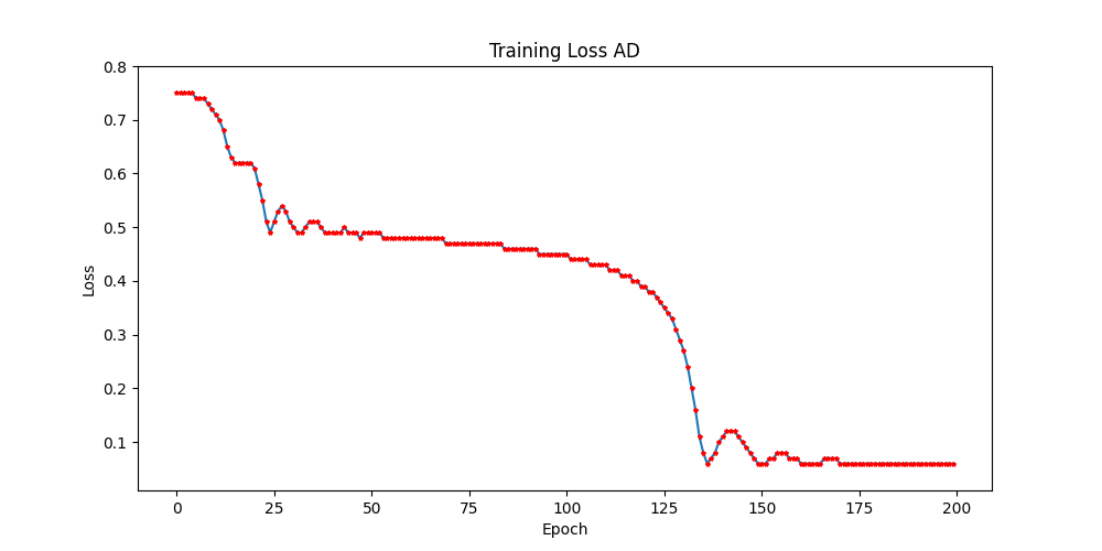
The coaching loss graph exhibits how the mannequin’s error decreases over 200 epochs with AdaHessian optimization.
Initially fast, the loss discount slows later, suggesting convergence. Fluctuations round epochs 100-150 point out attainable noise or studying fee changes. AdaHessian successfully optimizes the mannequin by adjusting studying steps utilizing second-order spinoff info.

Now Let’s visualize error or loss operate of our sigmoid neuron in Utilizing 2D and 3D Graphs .

2D Graphs

Right here we’re plotting the loss floor of the Neuron in 2nd:

• The contour strains symbolize ranges of the loss operate worth. The purple areas correspond to greater loss values, and the blue areas correspond to decrease loss values. Ideally, the optimization algorithm ought to transfer in the direction of the blue areas the place the loss is decrease.
• The black dot represents the present values of weight (w) and bias (b) at this epoch. Its place on the plot suggests the preliminary parameters earlier than coaching begins.
• As every epoch progresses with the AdaHessian optimizer updating weights and biases, the gradient steadily descends in the direction of the minima. The altering values of weights create a trajectory of optimization, regularly transferring in the direction of the minima, leading to a lower in error as effectively.

3D Graphs

Lets visualize the Loss operate of the neuron in 3D  for higher visualization.

It offers a visible illustration of the loss floor with respect to the load (w) and bias (b) of a single neuron mannequin, with the third axis representing the loss worth.

• Axes : The horizontal airplane represents the parameters—weight (w) on one axis and bias (b) on one other. The vertical axis represents the loss worth.
• Contourplot and Floor  : Beneath the floor, the contour plot is seen. It represents the identical info because the floor however from a top-down view. The contour strains assist to visualise the gradient (or slope) of the floor
• Optimization Path : The black line exhibits how our optimization course of strikes in the direction of the bottom level within the 3D plots. Within the 2D determine or floor of this , you’ll be able to see this because the purple line tracing the identical path downward in the direction of the minimal.

So the visualizations depict the loss floor of a sigmoid neuron utilizing 2D and 3D plots. Contour strains in 2D present completely different loss ranges, with purple for greater and blue for decrease losses.

The black dot represents preliminary parameters, and the optimization path demonstrates descent in the direction of decrease loss values. The 3D plot provides depth, illustrating the loss floor with weight, bias, and loss worth. 

Now After Analyzing outcomes let’s examine it with Adam with similar set of configuration however these consequence are extracted utilizing the pytorch body work for extra details about the implementation observe github hyperlink right here.

Lack of Adam and AdaHessian in Coaching Part

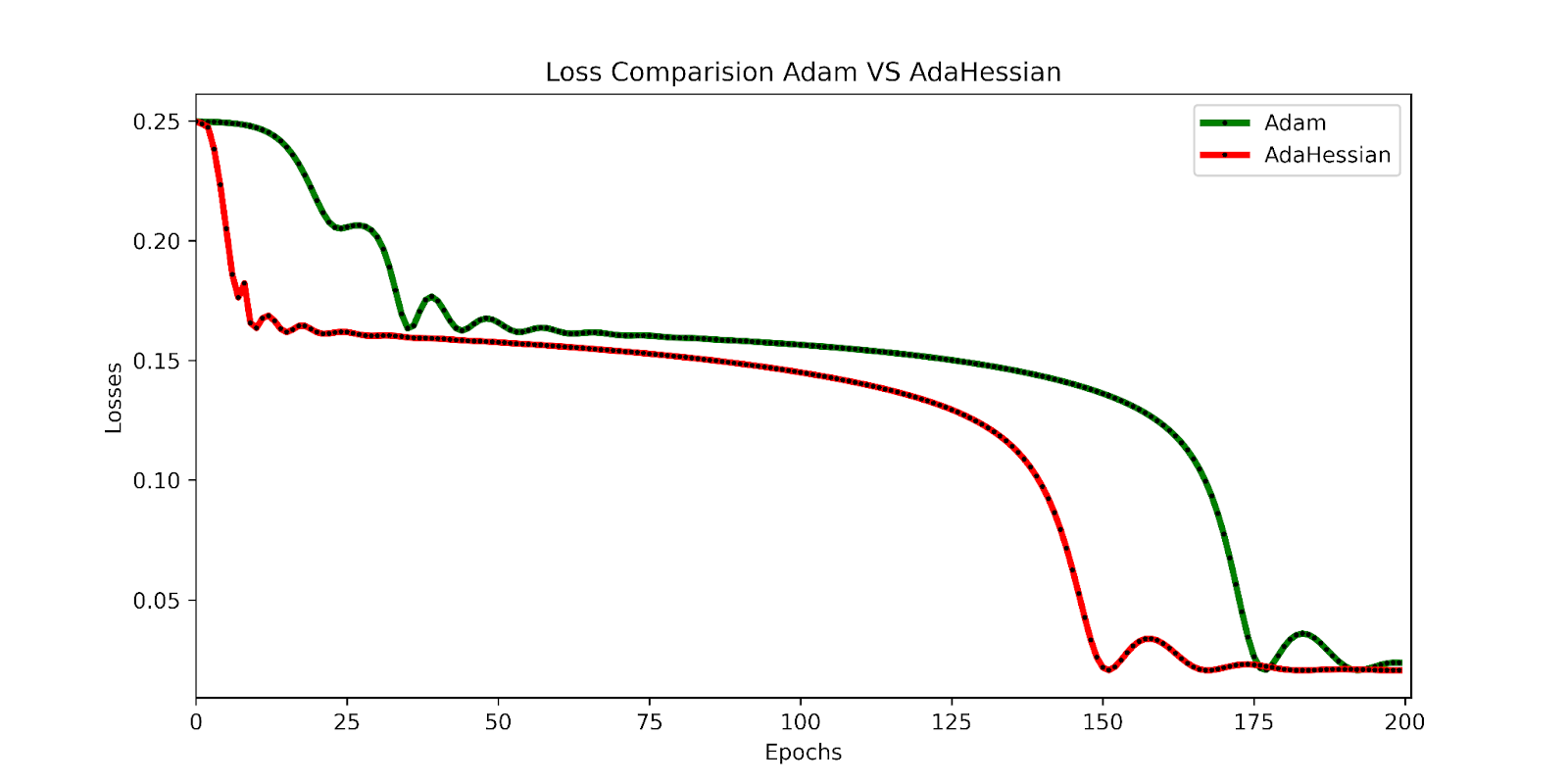
The AdaHessian loss stabilizes after 150 epochs, indicating that the optimization course of reaches a gradual state. Alternatively, the Adam loss continues to lower till it additionally stabilizes at 175 epochs, aligning with the AdaHessian loss development. This exhibits that AdaHessian successfully optimizes the mannequin by leveraging second-order spinoff info, which permits for exact changes in studying steps to attain optimum efficiency.

Lets Visualize this Comparability within the 2nd and 3d for the higher understanding of the optimization course of.

Visible Comparability in 2D Graphs 

On this  2D contour plot evaluating the loss floor traversal of two completely different optimization algorithms: Adam and AdaHessian. The axes w and b symbolize the load and bias parameters of a neuron, whereas the contour strains point out ranges of loss.

• Path Comparability : There are two paths marked on the plot, one for Adam (black) and one for AdaHessian (purple). These paths present the trajectory of the load and bias values as they’re up to date by their respective algorithms throughout coaching.
• Beginning Factors : Each paths begin on the similar level, indicated by the intersection of the 2 dotted strains, suggesting that each algorithms started with an identical preliminary situations for weight and bias.
• Algorithm Efficiency : Though it’s simply the preliminary level, the truth that each errors are equal means that at this very early stage in coaching, each optimizers are performing equivalently.
• Trajectories and Studying Dynamics : The paths present the path every optimizer is taking to reduce the loss.As we are able to see Over subsequent epochs, these paths illustrate how every optimizer navigates the loss floor otherwise, probably converging to completely different native minima or the worldwide minimal.
• Contour Gradients : The gradients of the contour strains give us a sign of how the loss adjustments with respect to w and b. Steeper gradients imply extra important adjustments in loss with small adjustments in parameters, whereas flatter areas point out much less sensitivity to parameter adjustments.
• Outcomes : As we are able to see that purple line(adahessian) transferring to the minima sooner or in much less epochs than the blackline(Adam).So Adahessian converging sooner than the Adam Although

To make this comparability extra comprehensible Lets analyse this comparability in 3D Plot.

Visible Comparability in 3D Graphs :

Contours in 3D plots present a complete view of the operate’s variations. On this evaluation, we give attention to the trajectory comparability between AdaHessian and Adam in a 3D plot.

• Trajectory Comparability: The 3D plot shows the trajectory of optimization for AdaHessian (purple) and Adam (inexperienced). AdaHessian’s trajectory exhibits a extra direct path in the direction of the minima in comparison with Adam.
• Optimization Dynamics: The contours within the 3D plot illustrate how the loss operate adjustments with completely different weight and bias mixtures. Steeper contours point out areas of fast loss change, whereas flatter contours symbolize slower adjustments.
• Outcomes Interpretation: From the 3D plot, it’s evident that AdaHessian converges sooner and follows a extra environment friendly path in the direction of the minimal loss in comparison with Adam.

This evaluation within the 3D plot offers a transparent visible understanding of how AdaHessian outperforms Adam when it comes to optimization pace and effectivity.

Conclusion

AdaHessian exhibits nice promise in addressing challenges confronted by conventional optimization strategies in deep studying. By leveraging second-order info, spatial averaging, and momentum methods, AdaHessian boosts optimization stability, quickens convergence, and navigates complicated landscapes extra successfully.

The evaluation of our plots revealed that AdaHessian’s loss stabilizes after 150 epochs. This means regular optimization, whereas AdamW continues to lower till stabilizing at 175 epochs. Visualizing the trajectories in 2D and 3D plots clearly demonstrated that AdaHessian converges sooner and takes a extra environment friendly path in the direction of minimal loss in comparison with AdamW.

This theoretical and sensible comparability underscores AdaHessian’s superiority in optimizing neural networks, particularly when it comes to convergence pace and effectivity. As deep studying fashions advance, algorithms like AdaHessian contribute considerably to bettering coaching dynamics, mannequin accuracy, and general efficiency. Embracing developments in optimization methods opens doorways to substantial progress in deep studying analysis and functions.

Key Takeaways

• AdaHessian is a second-order optimization algorithm designed to deal with challenges in conventional optimization strategies for deep studying.
• Second-order strategies face points like requiring full batch gradients, inaccurate Hessian approximations, and excessive computational and reminiscence overhead.
• The AdaHessian algorithm entails computing gradients, Hessian diagonals, spatially averaged diagonals, updating momentum phrases, and updating parameters for environment friendly optimization.
• Visualizing AdaHessian and Adam in 2D and 3D plots demonstrates AdaHessian’s sooner convergence and extra environment friendly trajectory in the direction of minimal loss.

Incessantly Requested Questions

Q1. What’s the distinction between first-order and second-order optimization? 

A. First-order strategies use gradient info, whereas second-order strategies like AdaHessian take into account each gradients and curvature (Hessian) info.

Q2. How does AdaHessian deal with challenges in optimization? 

A. AdaHessian addresses challenges reminiscent of computational value and inaccurate Hessian approximation through the use of environment friendly Hessian diagonal approximation and spatial methods.

Q3. What are the sensible advantages of implementing AdaHessian? 

A.  AdaHessian improves optimization stability, accelerates convergence, and handles complicated optimization landscapes successfully.  It’s notably helpful for large-scale deep studying fashions with high-dimensional parameter areas.

Q5. How can AdaHessian be in contrast with different optimization algorithms like AdamW? 

A. AdaHessian might be in contrast with different first-order and second-order strategies when it comes to convergence pace, stability, effectivity, and reminiscence utilization. Visualizing gradients and evaluating optimization trajectories can present insights into the efficiency variations between algorithms.