Freeze Panes in Excel?

Introduction

Microsoft Excel is among the many greatest applications for organizing and evaluating information. Certainly one of its most necessary options is the capability to freeze panes. This operate lets you choose sure rows or columns to maintain seen whereas searching the remainder of your spreadsheet, making information monitoring and comparability simpler. This submit will have a look at utilizing Excel’s Freeze Panes function and supply some useful ideas and examples.

Overview

• Freezing panes in Excel maintain particular rows or columns seen whereas scrolling via giant datasets, aiding in information monitoring and comparability.
• Enhances navigation, maintains header visibility, and simplifies information comparability inside intensive spreadsheets.
• Directions for freezing the highest row, first column, or a number of rows/columns utilizing the View tab and Freeze Panes possibility.
• Steps to take away frozen panes are via the View tab and the Unfreeze Panes possibility.
• Illustrations of utilizing Freeze Panes for information entry, comparative evaluation, and improved readability in numerous spreadsheet eventualities.
• Plan structure, use the Break up instrument for extra flexibility, and mix Freeze Panes with different Excel options like Filters and Conditional Formatting.

What’s Freezing Panes?

Excel has a operate known as “freezing panes” that lets you freeze particular rows and columns so that they keep seen when you navigate via the rest of the spreadsheet. That is fairly useful when working with monumental datasets and needing the headers or important columns to stay seen.

Use of Freeze Panes:

1. Higher Navigation: Transfer via big spreadsheets extra rapidly and precisely with out getting misplaced.
2. Preserve Visibility of Headers: Hold your column and row headers seen as you scroll via giant datasets.
3. Simpler Information Comparability: Keep in mind a very powerful data when evaluating information from numerous sections of your worksheet.

Additionally learn: Microsoft Excel for Information Evaluation

Freeze Panes in Excel?

Freezing the Prime Row

To maintain the highest row seen whereas scrolling down:

1. Open your Excel spreadsheet.
2. Go to the View tab on the Ribbon.
3. Click on on Freeze Panes within the Window group.
4. Choose Freeze Prime Row from the dropdown menu.

The highest row of your spreadsheet is now frozen and can stay seen as you scroll down.

Freezing the First Column

To maintain the primary column seen whereas scrolling to the fitting:

1. Open your Excel spreadsheet.
2. Go to the View tab on the Ribbon.
3. Click on on Freeze Panes within the Window group.
4. Choose the Freeze First Column from the dropdown menu.

The primary column of your spreadsheet is now frozen and can stay seen as you scroll horizontally.

Freezing A number of Rows or Columns

To freeze a number of rows or columns, or each:

1. Choose the cell under the rows and to the fitting of the columns you need to freeze. For instance, to freeze the primary two rows and the primary column, choose cell B3.
2. Go to the View tab on the Ribbon.
3. Click on on Freeze Panes within the Window group.
4. Choose Freeze Panes from the dropdown menu.

The rows above and columns to the left of your chosen cell are actually frozen.

Unfreezing Excel Panes

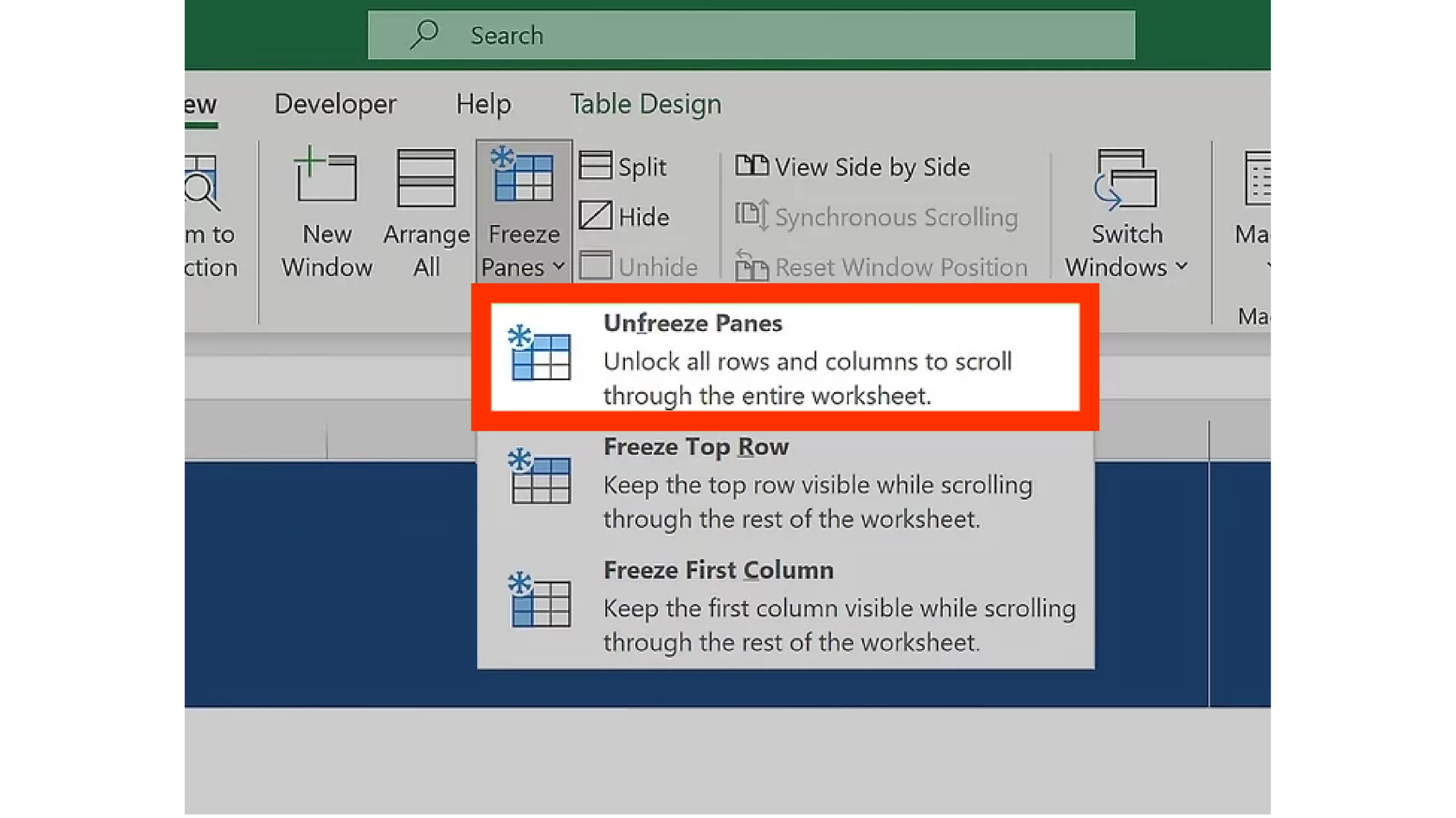
If it’s worthwhile to unfreeze the panes:

1. Go to the View tab on the Ribbon.
2. Click on on Freeze Panes within the Window group.
3. Choose Unfreeze Panes from the dropdown menu.

It will take away all frozen panes in your spreadsheet.

Additionally learn: A Complete Information on Superior Microsoft Excel for Information Evaluation

Sensible Examples of Freezing Panes in Excel

Listed here are the examples:

Instance 1: Freezing the Prime Row for Information Entry

Let’s say you could have a giant dataset with headers (e.g., Title, Age, Division) on the primary row, every representing a definite merchandise. By freezing the highest row, you may be sure that the headers keep displayed when you enter information into the next rows.

Instance 2: Freezing the First Column for Comparative Evaluation

Let’s say you could have a monetary report that lists a number of monetary metrics within the following columns and months within the first column. Evaluating the primary column is less complicated when it’s frozen since you may scroll via the metrics and all the time see the month.

Instance 3: Freezing Each Rows and Columns for Enhanced Readability

If you navigate a spreadsheet with each column headings and row labels—for instance, a gross sales report with product names within the first column and gross sales areas within the high row freezing the primary column and the highest row makes it simpler to take care of monitor of each dimensions of your information.

Suggestions for Utilizing Freeze Panes Successfully

Listed here are ideas for utilizing freeze:

1. Plan Your Format: Decide which rows and columns are essential for navigation and comparability earlier than freezing panes.
2. Use Break up for Extra Flexibility: In case you want much more freedom, you should utilize the Break up instrument (positioned below the View tab) to create separate scrollable sections.
3. Incorporate with Further Options: Mix Freeze Panes with different Excel capabilities, reminiscent of Filters, Tables, and Conditional Formatting, to enhance your information evaluation workflow.

Conclusion

Excel’s freezing panes are an easy however efficient approach that improves your potential to discover and analyze large datasets. You possibly can protect context and improve productiveness by making key rows and columns seen. Utilizing Excel’s Freeze Panes instrument will enhance your productiveness, whether or not you’re getting into information, evaluating metrics, or studying reviews.

Regularly Requested Questions