A Complete Forecasting Strategy 📈🕵🏼‍♂️👨🏼‍💻

Machine Studying (ML) is a strong software to foretell gross sales or perceive the behavioral sample underlying the information. In an period the place information is the gas to rework any enterprise and revolutionize its gross sales methods, on the forefront of this transformation is predictive evaluation empowered by the capabilities of machine studying. This dynamic mixture not solely permits organizations to make sense of huge datasets but in addition empowers them to forecast gross sales developments, optimize decision-making, and in the end drive income development.

Machine studying algorithms will be educated to acknowledge patterns and correlations inside the information, enabling organizations to foretell future outcomes with a excessive diploma of accuracy. Whether or not it is forecasting buyer demand, figuring out high-value leads, or optimizing pricing methods, predictive evaluation pushed by machine studying gives a data-driven basis for decision-makers.

On this article, we are going to attempt to forecast the gross sales of a retailer utilizing Kaggle’s dataset. The principle goal of this problem is to create an ML mannequin to foretell the gross sales information for future months.

Gross sales forecasting entails the estimation of future gross sales utilizing predictive fashions or tailored strategies, with various levels of accuracy. This apply necessitates the consideration of each qualitative and quantitative variables within the course of.

Gross sales forecasting entails understanding the sample of enterprise by utilizing know-how reminiscent of ML. This entails making a mannequin which takes in great amount of historic information on which future patterns are predicted.

Understanding the Significance of Future Gross sales Forecasting

Gross sales forecasting performs a vital position in companies choice making by offering insights into what to anticipate from the approaching months. Listed here are just a few key factors to know why gross sales forecasting is beneficial in enterprise:

• Strategic Determination Making: Gross sales forecasting aids in strategic decision-making by offering insights into anticipated gross sales. This in flip helps any enterprise to be ready by establishing practical targets, allocating satisfactory sources, and planning for development.
• Advertising Technique: Forecasting generates vital information for companies. This data can assist in making strategic choices reminiscent of allocating advertising budgets successfully, directing efforts towards the suitable target market, and evaluating the long run gross sales impression of promoting campaigns.
• Monetary Planning: Future gross sales forecasts contribute to efficient monetary planning. Companies can align their budgets with anticipated income, handle money stream, and make knowledgeable monetary choices.
• Threat Administration: Forecasting permits companies to determine potential dangers and uncertainties. By understanding market dynamics, companies can develop methods to mitigate dangers related to financial fluctuations, altering shopper conduct, or exterior elements.

Challenges

Gross sales forecasting addresses the efficiency and profitability necessities of organizations, making it a vital ingredient in an organization’s gross sales technique, regardless of its trade or sector. When discussing the strategic facets of gross sales forecasting, we’re primarily specializing in the challenges that, if resolved, would allow an organization to implement its gross sales technique with larger confidence.

• Market Uncertainty: Market situations are sometimes unpredictable, making it difficult to precisely forecast gross sales. Exterior elements reminiscent of geopolitical occasions, financial downturns, or pure disasters can considerably impression shopper conduct.
• Seasonal Variations: Many industries expertise seasonal fluctuations in demand. Forecasting turns into complicated when coping with the cyclical nature of sure services or products, requiring companies to account for these variations.
• Altering Client Habits: Fast modifications in shopper preferences and conduct can disrupt conventional forecasting fashions. Shifts in shopping for patterns influenced by technological developments or cultural modifications pose challenges for correct predictions.
• Aggressive Dynamics: The aggressive panorama is dynamic, with new entrants, evolving methods, and altering market shares. Predicting the actions of rivals and their impression on gross sales provides an extra layer of complexity.

Completely different Machine Studying Strategies for Gross sales Forecasting

Listed here are some frequent machine studying strategies utilized in gross sales forecasting:

• Linear Regression: Linear regression fashions set up a linear relationship between the enter options and the goal variable (gross sales). It’s appropriate for situations the place the connection is predicted to be roughly linear.
• Time Collection Evaluation: Time sequence strategies, reminiscent of ARIMA (AutoRegressive Built-in Transferring Common) or Exponential Smoothing, are particularly designed for forecasting based mostly on historic time-ordered information. These strategies take into account patterns and seasonality within the time sequence.
• Determination Timber: Determination timber are tree-like fashions that cut up information based mostly on enter options, making a algorithm for predicting the goal variable. They’re intuitive and might deal with each numerical and categorical information.
• Random Forest: Random Forest is an ensemble technique that builds a number of choice timber utilizing random characteristic choice with alternative and combines their predictions. It typically performs properly and is powerful to overfitting.
• Neural Networks (Deep Studying): Neural networks, particularly deep studying fashions, can seize complicated patterns in information. Recurrent Neural Networks (RNNs) and Lengthy Brief-Time period Reminiscence networks (LSTMs) are generally used for sequential information like time sequence.
• Ok-Nearest Neighbors (KNN): KNN is a straightforward algorithm that classifies information factors based mostly on the bulk class of their nearest neighbors. It may be tailored for regression duties in gross sales forecasting.
• XGBoost: XGBoost is an environment friendly and scalable implementation of gradient boosting. It’s significantly efficient in dealing with massive datasets and has been profitable in numerous machine studying competitions.
• Ensemble Strategies: Ensemble strategies, together with bagging and boosting, mix a number of fashions to enhance total efficiency. Bagging strategies like Bootstrap Aggregating (Bagging) and boosting strategies like AdaBoost are generally used.

It’s common to experiment with a number of strategies to find out which one performs finest for a specific situation.

Gross sales Forecasting Utilizing Python on the Paperspace Platform

Right here we are going to attempt to use a Kaggle’s gross sales dataset and use numerous ML methods to foretell the gross sales for future information. We now have offered the CSV for the reader’s comfort.

Please click on the hyperlink to entry your entire pocket book and entry the complete code. On this article we’re offering a complete code overview.

1. Importing the required libraries

#import the libraries
import pandas as pd
import numpy as np
from sklearn.model_selection import RandomizedSearchCV
import joblib
import os
import matplotlib.pyplot as plt
import seaborn as sns
import warnings
import pickle

from sklearn.linear_model import LinearRegression
from sklearn.ensemble import RandomForestRegressor
import xgboost as xgb
from sklearn.metrics import mean_absolute_error, mean_squared_error, r2_score
warnings.filterwarnings('ignore')

# settings to show all columns
pd.set_option("show.max_columns", None)

2. Loading and Exploration of the Information

Allow us to begin by loading the datasets to carry out the essential Exploratory Information Evaluation (EDA) on the information.

#operate that can be used for the extraction of a CSV file after which changing it to pandas dataframe
def load_data(file_name):  
    """Returns a pandas dataframe from a csv file."""  
    return pd.read_csv(file_name)
train_df = load_data('practice.csv')
test_df = load_data('check.csv')
syb_df = load_data('sample_submission.csv')

The beneath piece of code gives the time interval of the obtainable information, offered for the mannequin coaching and testing information

def sales_period(information):  
    """Time interval of practice dataset:"""  
  
    print(f'time interval begins from :{information["date"].min()}, and ends in :{information["date"].max()}')
sales_period(train_df)
sales_period(test_df)

time interval begins from :2013-01-01, and ends in :2017-12-31
time interval begins from :2018-01-01, and ends in :2018-03-31

3. Primary EDA

def sales_per_store(information):
    
    sales_by_store = information.groupby('retailer')['sales'].sum().reset_index() 
    fig, ax = plt.subplots(figsize=(8,6)) 
    sns.barplot(sales_by_store, x="retailer", y="gross sales", estimator="sum", errorbar=None)
    ax.set(xlabel = "Retailer Id", ylabel = "Sum of Gross sales", title = "Complete Gross sales Per Retailer")   
     
    return sales_by_store, ax

sales_per_store(train_df)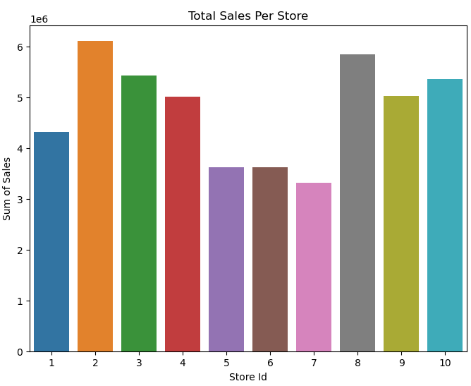

def sales_by_dt(information):
    information['date'] = pd.to_datetime(information['date'])
    sales_by_date = information.groupby('date')['sales'].sum().reset_index()

    #show the outcomes
    return sales_by_date

sales_by_date = sales_by_dt(train_df)

Plot the gross sales to know the gross sales sample over time

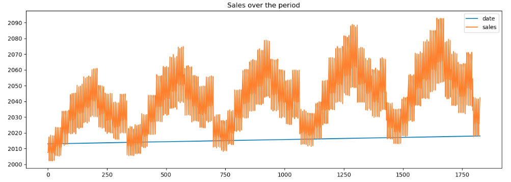
As evident from the plot we discover that the gross sales have elevated through the years for all of the shops.

4. Information Preprocessing together with EDA at every step

The beneath code snippet takes the unique coaching DataFrame (train_df), teams the information by date, sums the gross sales for every date, converts the index to datetime format, drops pointless columns. This transformation is beneficial when analyzing total gross sales developments each day, with out contemplating particular person shops or objects.

#Mixture Every day Gross sales Information by Date from Coaching Dataset
train_dt_sales = train_df.groupby('date').sum('gross sales')
train_dt_sales.index = pd.to_datetime(train_dt_sales.index)
train_dt_sales = train_dt_sales.drop(['store','item'], axis=1)
train_dt_sales.head()

DataFrame is cut up into two components: the coaching set (practice) and the check set (check). On this case, all information earlier than January 1, 2017, is taken into account the coaching set, whereas information from and after January 1, 2017, is taken into account the check set.

#creates a practice/check cut up of time sequence information, plots the coaching and check units on a single graph, and provides a visible indicator of the cut up level
practice = train_dt_sales.loc[train_dt_sales.index < '01-01-2017']
check = train_dt_sales.loc[train_dt_sales.index >= '01-01-2017']

fig, ax = plt.subplots(figsize=(15, 5))
practice.plot(ax=ax, label="Coaching Set", title="Practice/Check Cut up information")
check.plot(ax=ax, label="Check Set")
ax.axvline('01-01-2017', coloration="Grey", ls="--")
ax.legend(['Training Set', 'Test Set'])
plt.present()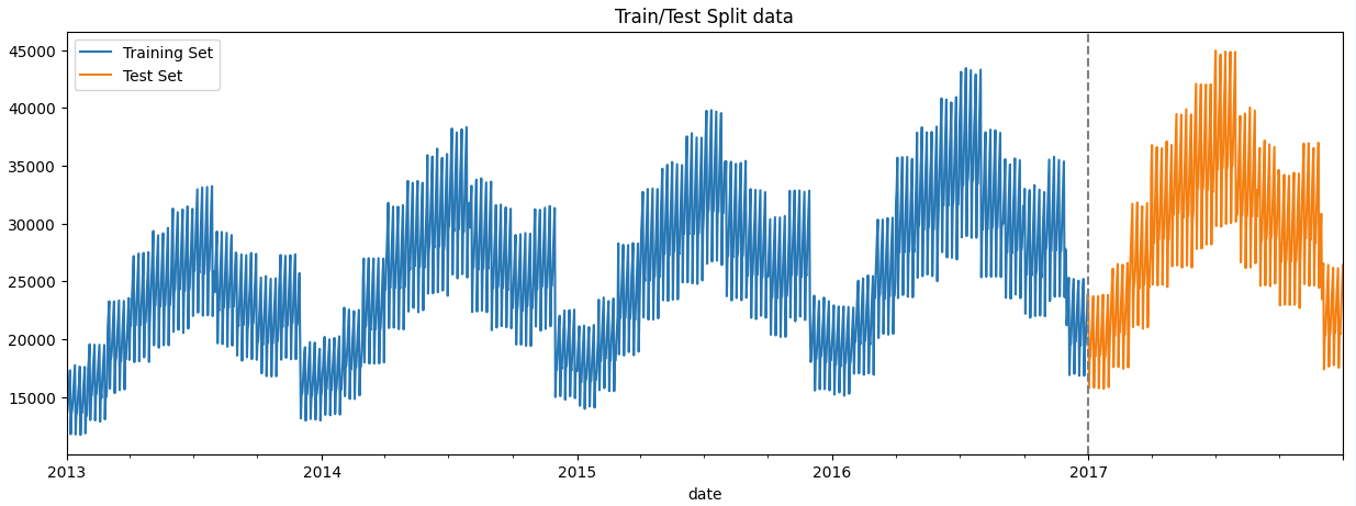

Within the dataset we’re supplied with the date column which can be utilized to extract options reminiscent of ‘day_of_week’, ‘day_of_year’, ‘quarter’, and so on.

#creating options from the prevailing options reminiscent of day of week, hour, month
def create_features(df):
    """
    Creating time sequence options based mostly on dataframe index.
    """
    df = df.copy()
    # df['hour'] = df.index.hour
    df['dayofweek'] = df.index.dayofweek
    df['quarter'] = df.index.quarter
    df['month'] = df.index.month
    df['year'] = df.index.yr
    df['dayofyear'] = df.index.dayofyear
    df['dayofmonth'] = df.index.day
    df['weekofyear'] = df.index.isocalendar().week
    return df

train_dt_sales = create_features(train_dt_sales)

The beneath plots helps to analyse the gross sales information over the week and month

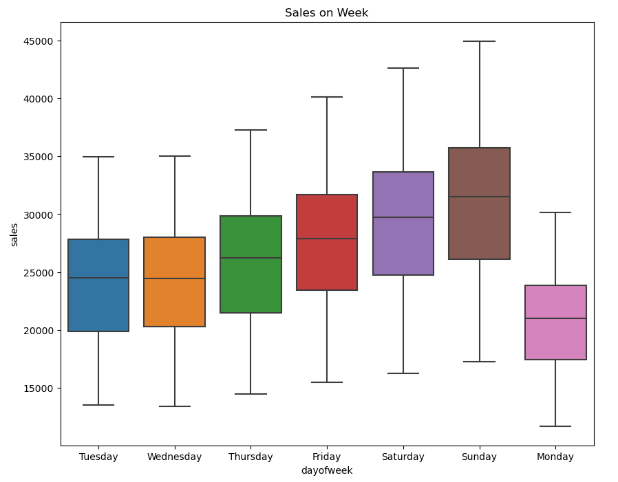
Gross sales sometimes exhibit an upward pattern ranging from Friday, attain their peak on Sunday, after which expertise a decline on Monday. This sample is influenced by the elevated gross sales that generally happen over the weekends.

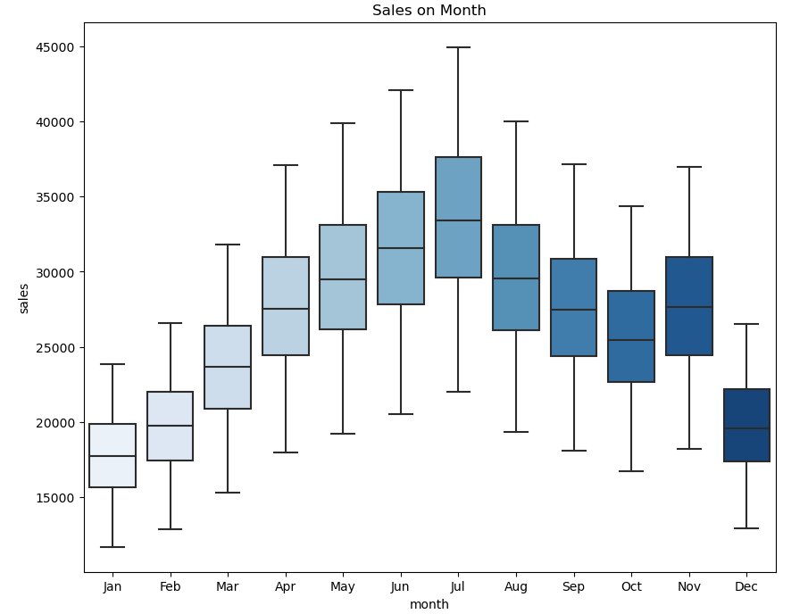
Within the plot above we discover {that a} sturdy shift happens from the month of April and begins declining from August. Moreover, the plot reveals an upward spike within the month of November.

5. Mannequin constructing

We purpose to make use of three distinct fashions—Linear Regression, Random Forest, and XGBoost—to forecast gross sales utilizing the coaching dataset. The most effective mannequin amongst these can be utilized to foretell gross sales for the check information.

Allow us to begin with constructing a linear regression mannequin to foretell the gross sales.

Linear Regression

Linear regression is a supervised ML algorithm that gives a linear relationship between a dependent and an unbiased variable by drawing a finest match line between the 2 variables.

# match a linear regression mannequin
linreg_model = LinearRegression()
linreg_model.match(X_train, y_train)

#predict on the check(future) information
check['prediction_lr'] = linreg_model.predict(X_test)

The beneath code calculates and prints three efficiency metrics to guage the efficiency of a Linear Regression mannequin on the check information.

#metrics to confirm the mannequin
linreg_rmse = np.sqrt(mean_squared_error(check['sales'], check['prediction_lr']))
linreg_mae = mean_absolute_error(check['sales'], check['prediction_lr'])
linreg_r2 = r2_score(check['sales'], check['prediction_lr'])
print('Linear Regression RMSE: ', linreg_rmse)
print('Linear Regression MAE: ', linreg_mae)
print('Linear Regression R2 Rating: ', linreg_r2)

Root Imply Squared Error (RMSE): The mean_squared_error operate from sklearn.metrics is used to calculate the imply squared error between the precise gross sales (check['sales']) and the anticipated gross sales (check['prediction_lr']) by the Linear Regression mannequin. The result’s then square-rooted to acquire the RMSE.

Imply Absolute Error (MAE): The mean_absolute_error operate is used to calculate the imply absolute error between the precise and predicted gross sales. It gives the typical absolute distinction between the anticipated and precise values.

R-squared (R2) Rating: The r2_score operate calculates the R-squared rating, which signifies the proportion of the variance within the dependent variable (gross sales) that’s predictable from the unbiased variable (prediction_lr). It measures the goodness of match of the mannequin.

Random Forest

Random Forest is an ensemble studying technique used for each classification and regression duties in machine studying. Random Forest builds a number of choice timber throughout coaching. Every tree is educated on a random subset of the options and a random subset of the coaching information. This randomness helps forestall overfitting and contributes to the mannequin’s robustness.

# biuld a random forest mannequin 
rf_model = RandomForestRegressor(n_estimators=100, max_depth=20)
rf_model.match(X_train, y_train)

check['prediction_rf'] = rf_model.predict(X_test)
#mannequin analysis metrics
rf_rmse = np.sqrt(mean_squared_error(check['sales'], check['prediction_rf']))
rf_mae = mean_absolute_error(check['sales'], check['prediction_rf'])
rf_r2 = r2_score(check['sales'], check['prediction_rf'])
print('Random Forest RMSE: ', rf_rmse)
print('Random Forest MAE: ', rf_mae)
print('Random Forest R2 Rating: ', rf_r2)

The offered code snippet builds a Random Forest mannequin for regression utilizing the RandomForestRegressor from scikit-learn.

XGBoost

XGBoost, quick for eXtreme Gradient Boosting, is a strong and extensively used machine studying algorithm that belongs to the gradient boosting household. It’s significantly in style for its excessive efficiency, effectivity, and flexibility in quite a lot of machine studying duties, together with classification, regression, and rating issues.

# xgboost mannequin 

reg = xgb.XGBRegressor(base_score=0.5, booster="gbtree",    
                       n_estimators=1000,
                       early_stopping_rounds=50,
                       goal="reg:linear",
                       max_depth=3,
                       learning_rate=0.01)
reg.match(X_train, y_train,
        eval_set=[(X_train, y_train), (X_test, y_test)],
        verbose=100)

xg_rmse = np.sqrt(mean_squared_error(check['sales'], check['prediction_xg']))
xg_mae = mean_absolute_error(check['sales'], check['prediction_xg'])
xg_r2 = r2_score(check['sales'], check['prediction_xg'])
print('Random Forest RMSE: ', xg_rmse)
print('Random Forest MAE: ', xg_mae)
print('Random Forest R2 Rating: ', xg_r2)

Outcomes

When evaluating numerous machine studying fashions, it is necessary to think about a number of elements for comparability.

In our particular case, we are going to particularly deal with evaluating fashions utilizing the Root Imply Squared Error (RMSE), Imply Absolute Error (MAE), and R-squared (R2) Rating.

In our case, we are going to use a random forest mannequin to foretell the gross sales for the check information.

# drop the pointless columns and biuld the mannequin
test_df.drop(['id','store','item'], axis=1, inplace=True)
test_df.index = pd.to_datetime(test_df.date)
to_predict_test_feature = create_features(test_df)
to_predict_test_feature = to_predict_test_feature[FEATURES]
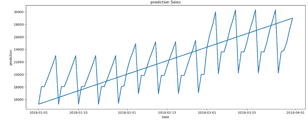
to_predict_test_feature['prediction'] = reg.predict(to_predict_test_feature)
to_predict_test_feature.head()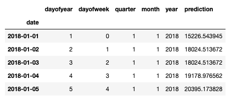

Plot the gross sales prediction

Conclusion

On this tutorial, we utilized the capabilities of machine studying for gross sales forecasting, a barely completely different method from typical strategies just like the ARIMA mannequin. Nonetheless, this method proves extremely efficient in precisely predicting gross sales. The utilization of superior algorithms, reminiscent of XGBoost and Random Forest, permits companies to extract priceless insights from huge datasets, enhancing their predictive capabilities. The importance of correct gross sales forecasting extends past mere numerical predictions; it turns into a strategic software that empowers organizations to optimize useful resource allocation, refine advertising methods, and fortify decision-making processes.

We strongly encourage you to execute the pocket book and discover its functionalities. Our intention is to construct a robust basis framework for the mannequin and its experiments, serving as a place to begin on your exploration.

Thanks a lot for studying!!

References