Simulating Life within the Browser: Making a Residing Particle System for the UntilLabs Web site

Till Labs is advancing probably the most significant issues in fashionable healthcare: preserving the potential of life. So when at basement.studio we got down to design their homepage, we didn’t need an summary animation, we wished one thing that felt actual, one thing that echoed the science on the core of their work. The concept was easy however formidable: take an actual {photograph} of individuals and reconstruct it as a dwelling particle system — a digital scene formed by actual information, pure movement, and physics-driven habits. A system that feels alive as a result of it’s constructed from life itself.

Right here’s how we made it occur.

Let’s break down the method:

Be taught fashionable net animation utilizing GSAP 3 with 34 hands-on video classes and sensible tasks — good for all ability ranges.

Test it out

1. Planting the First Pixels: A Easy Particle Discipline

Earlier than realism can exist, it wants a stage. A spot the place hundreds of particles can dwell, transfer, and be manipulated effectively.

This results in one important query:

How will we render tens of hundreds of unbiased factors at excessive body charges?

To realize this, we constructed two foundations:

• A scalable particle system utilizing GL_POINTS
• A fashionable render pipeline constructed on FBOs and a fullscreen QuadShader

Collectively, they type a versatile canvas for all future results.

A Easy, Scalable Particle Discipline

We generated 60,000 particles inside a sphere utilizing correct spherical coordinates. This gave us:

• A pure, volumetric distribution
• Sufficient density to characterize a high-res picture later
• Maintains a relentless 60 FPS.

const geo = new THREE.BufferGeometry();
const positions = new Float32Array(rely * 3);
const scales = new Float32Array(rely);
const randomness = new Float32Array(rely * 3);

for (let i = 0; i < rely; i++) {
  const i3 = i * 3;

  // Uniform spherical distribution
  const theta = Math.random() * Math.PI * 2.0;
  const phi = Math.acos(2.0 * Math.random() - 1.0);
  const r = radius * Math.cbrt(Math.random());

  positions[i3 + 0] = r * Math.sin(phi) * Math.cos(theta);
  positions[i3 + 1] = r * Math.sin(phi) * Math.sin(theta);
  positions[i3 + 2] = r * Math.cos(phi);

  scales[i] = Math.random() * 0.5 + 0.5;
  randomness[i3 + 0] = Math.random();
  randomness[i3 + 1] = Math.random();
  randomness[i3 + 2] = Math.random();
}

geo.setAttribute("place", new THREE.BufferAttribute(positions, 3));
geo.setAttribute("aScale", new THREE.BufferAttribute(scales, 1));
geo.setAttribute("aRandomness", new THREE.BufferAttribute(randomness, 3));

Rendering With GL_POINTS + Customized Shaders

GL_POINTS permits us to attract each particle in one draw name, good for this scale.

Vertex Shader — GPU-Pushed Movement

uniform float uTime;

attribute float aScale;
attribute vec3 aRandomness;

various vec3 vColor;

void principal() {
  vec4 modelPosition = modelMatrix * vec4(place, 1.0);

  // GPU animation utilizing per-particle randomness
  modelPosition.xyz += vec3(
    sin(uTime * 0.5 + aRandomness.x * 10.0) * aRandomness.x * 0.3,
    cos(uTime * 0.3 + aRandomness.y * 10.0) * aRandomness.y * 0.3,
    sin(uTime * 0.4 + aRandomness.z * 10.0) * aRandomness.z * 0.2
  );

  vec4 viewPosition = viewMatrix * modelPosition;
  gl_Position = projectionMatrix * viewPosition;

  gl_PointSize = uSize * aScale * (1.0 / -viewPosition.z);
  vColor = vec3(1.0);
}

various vec3 vColor;

void principal() {
  float d = size(gl_PointCoord - 0.5);
  float alpha = pow(1.0 - smoothstep(0.0, 0.5, d), 1.5);
  gl_FragColor = vec4(vColor, alpha);
}

We render the particles into an off-screen FBO so we are able to deal with your entire scene as a texture. This lets us apply colour grading, results, and post-processing with out touching the particle shaders, holding the system versatile and simple to iterate on.

Three elements work collectively:

1. createPortal: Isolates the 3D scene into its personal THREE.Scene
2. FBO (Body Buffer Object): Captures that scene as a texture
3. QuadShader: Renders a fullscreen quad with post-processing

// Create remoted scene
const [contentScene] = useState(() => {
  const scene = new THREE.Scene();
  scene.background = new THREE.Shade("#050505");
  return scene;
});

return (
  <>
    {/* 3D content material renders to contentScene, not the principle scene */}
    {createPortal(kids, contentScene)}
    
    {/* Put up-processing renders to principal scene */}
    <QuadShader program={postMaterial} renderTarget={null} />
  </>
);

Utilizing @react-three/drei’s useFBO, we create a render goal that matches the display screen:

const sceneFBO = useFBO(fboWidth, fboHeight, {
  minFilter: THREE.LinearFilter,
  magFilter: THREE.LinearFilter,
  format: THREE.RGBAFormat,
  sort: THREE.HalfFloatType,  // 16-bit for HDR headroom
});

useFrame((state, delta) => {
  const gl = state.gl;

  // Step 1: Render 3D scene to FBO
  gl.setRenderTarget(sceneFBO);
  gl.clear();
  gl.render(contentScene, digital camera);
  gl.setRenderTarget(null);

  // Step 2: Feed FBO texture to post-processing
  postUniforms.uTexture.worth = sceneFBO.texture;

  // Step 3: QuadShader renders to display screen (dealt with by QuadShader element)
}, -1);  // Precedence -1 runs BEFORE QuadShader's precedence 1

2. Nature Is Fractal

Borrowing Movement from Nature: Brownian Motion

Now that the particle system is in place, it’s time to make it behave like one thing actual. In nature, molecules don’t transfer in straight strains or observe a single drive — their movement comes from overlapping layers of randomness. That’s the place fractal Brownian movement is available in.

Through the use of fBM in our particle system, we weren’t simply animating dots on a display screen; we have been borrowing the identical logic that shapes molecular movement.

float random(vec2 st) {
  return fract(sin(dot(st.xy, vec2(12.9898, 78.233))) * 43758.5453123);
}

// 2D Worth Noise - Based mostly on Morgan McGuire @morgan3d
// https://www.shadertoy.com/view/4dS3Wd
float noise(vec2 st) {
  vec2 i = flooring(st);
  vec2 f = fract(st);

  // 4 corners of the tile
  float a = random(i);
  float b = random(i + vec2(1.0, 0.0));
  float c = random(i + vec2(0.0, 1.0));
  float d = random(i + vec2(1.0, 1.0));

  // Easy interpolation
  vec2 u = f * f * (3.0 - 2.0 * f);

  return combine(a, b, u.x) +
         (c - a) * u.y * (1.0 - u.x) +
         (d - b) * u.x * u.y;
}

// Fractal Brownian Movement - layered noise for pure variation
float fbm(vec2 st, int octaves) {
  float worth = 0.0;
  float amplitude = 0.5;
  vec2 shift = vec2(100.0);

  // Rotation matrix to cut back axial bias
  mat2 rot = mat2(cos(0.5), sin(0.5), -sin(0.5), cos(0.5));

  for (int i = 0; i < 6; i++) {
    if (i >= octaves) break;
    worth += amplitude * noise(st);
    st = rot * st * 2.0 + shift;
    amplitude *= 0.5;
  }

  return worth;
}

// Curl Noise
vec2 curlNoise(vec2 st, float time) {
  float eps = 0.01;

  // Pattern FBM at offset positions
  float n1 = fbm(st + vec2(eps, 0.0) + time * 0.1, 4);
  float n2 = fbm(st + vec2(-eps, 0.0) + time * 0.1, 4);
  float n3 = fbm(st + vec2(0.0, eps) + time * 0.1, 4);
  float n4 = fbm(st + vec2(0.0, -eps) + time * 0.1, 4);

  // Calculate curl (perpendicular to gradient)
  float dx = (n1 - n2) / (2.0 * eps);
  float dy = (n3 - n4) / (2.0 * eps);

  return vec2(dy, -dx);
}

3. The Massive Problem: From Actuality to Knowledge

With movement solved, the subsequent step was to present the particles one thing significant to characterize:

An actual {photograph}, reworked right into a discipline of factors.

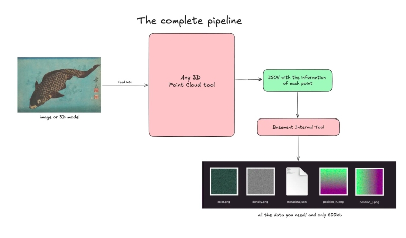
From {Photograph} → Level Cloud → JSON

By way of any 3D Level Cloud software, we:

1. Took a high-res actual picture / 3D mannequin
2. Generated a level cloud
3. Exported every pixel/level as JSON:

This labored, however resulted in a 20 MB JSON — far too heavy.

The Resolution: Textures as Knowledge

As a substitute of delivery JSON, we saved particle information inside textures. Utilizing an inner software we have been capable of cut back the 20MB JSON to:

A tiny metadata file describes the format:

{
  "width": 256,
  "top": 256,
  "particleCount": 65536,
  "bounds": {
    "min": [-75.37, 0.0, -49.99],
    "max": [75.37, 0.65, 49.99]
  },
  "precision": "16-bit (break up throughout excessive/low textures)"
}

All recordsdata mixed? ~604 KB — a large discount.

Now we are able to load these pictures within the code and use the vertex and fragment shaders to characterize the mannequin/picture on display screen. We ship them as uniforms to the vertex shader, load and mix them.

  //... earlier code 
  
 // === 16-BIT POSITION RECONSTRUCTION ===
  // Pattern each excessive and low byte place textures
  vec3 sampledPositionHigh = texture2D(uParticlesPositionHigh, aParticleUv).xyz;
  vec3 sampledPositionLow = texture2D(uParticlesPositionLow, aParticleUv).xyz;
  
  // Convert normalized RGB values (0-1) again to byte values (0-255)
  float colorRange = uTextureSize - 1.0;
  vec3 highBytes = sampledPositionHigh * colorRange;
  vec3 lowBytes = sampledPositionLow * colorRange;
  
  // Reconstruct 16-bit values: (excessive * 256) + low for every XYZ channel
  vec3 position16bit = vec3(
    (highBytes.x * uTextureSize) + lowBytes.x,
    (highBytes.y * uTextureSize) + lowBytes.y,
    (highBytes.z * uTextureSize) + lowBytes.z
  );
  
  // Normalize 16-bit values to 0-1 vary
  vec3 normalizedPosition = position16bit / uParticleCount;
  
  // Remap to world coordinates
  vec3 particlePosition = remapPosition(normalizedPosition);

  // Pattern colour from texture
  vec3 sampledColor = texture2D(uParticlesColors, aParticleUv).rgb;
  vColor = sampledColor;
  
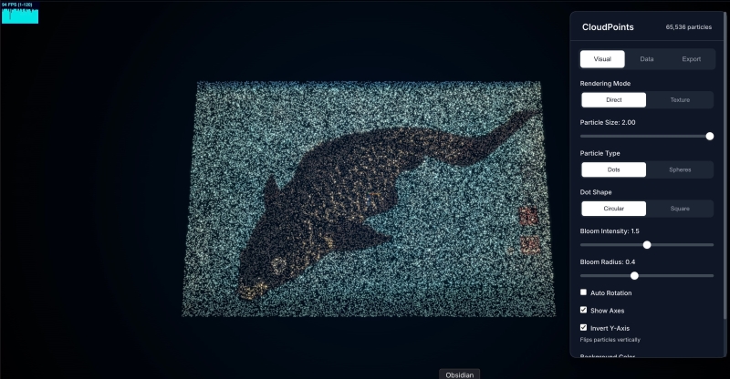
  //...and so on

Mix all collectively, add some tweaks to regulate every parameter of the factors, and voilà!

You may see the dwell demo right here.

4. Tweaking the Particles With Shaders

Due to the earlier implementation utilizing render targets and FBO, we are able to simply add one other render goal for post-processing results. We additionally added a LUT (lookup desk) for colour transformation, permitting designers to swap the LUT texture as they need—the modifications apply on to the ultimate consequence.

Life is now preserved and displayed on the net. The total image comes collectively: an actual {photograph} damaged into information, rebuilt by way of physics, animated with layered noise, and delivered by way of a rendering pipeline designed to remain quick, versatile, and visually constant. Each step, from the particle discipline to the information textures, the pure movement, the LUT-driven artwork path, feeds the identical purpose we set at first: make the expertise really feel alive.