What are the Completely different Elements of Diffusion Fashions?

Introduction

Synthetic intelligence has revolutionized due to Steady Diffusion, which makes producing high-quality photos from noise or textual content descriptions doable. A number of important components come collectively on this potent generative mannequin to create superb visible results. The 5 predominant elements of Diffusion Fashions—the ahead and reverse processes, the noise schedule, positional encoding, and neural community structure—will all be lined on this article.

We’ll implement elements of diffusion fashions as we undergo the article. We might be utilizing the Vogue MNIST Dataset for this. 

Overview

• Uncover how Steady Diffusion transforms AI picture technology, bringing high-quality visuals from mere noise or textual content descriptions.
• Learn the way photos degrade to noise, coaching AI fashions to grasp the artwork of visible reconstruction.
• Discover how AI reconstructs high-quality photos from noise, reversing the degradation course of step-by-step.
• Perceive the position of distinctive vector representations in guiding AI by various noise ranges throughout picture technology.
• Delve into the symmetrical encoder-decoder construction of UNet, which excels at producing advantageous particulars and world buildings.
• Look at the important noise schedule in diffusion fashions, balancing technology high quality and computational effectivity for high-fidelity AI outputs.

Ahead Diffusion Course of

The ahead course of is the preliminary stage of Steady Diffusion, the place a picture is progressively remodeled into noise. This course of is essential for coaching the mannequin to know how photos degrade over time.

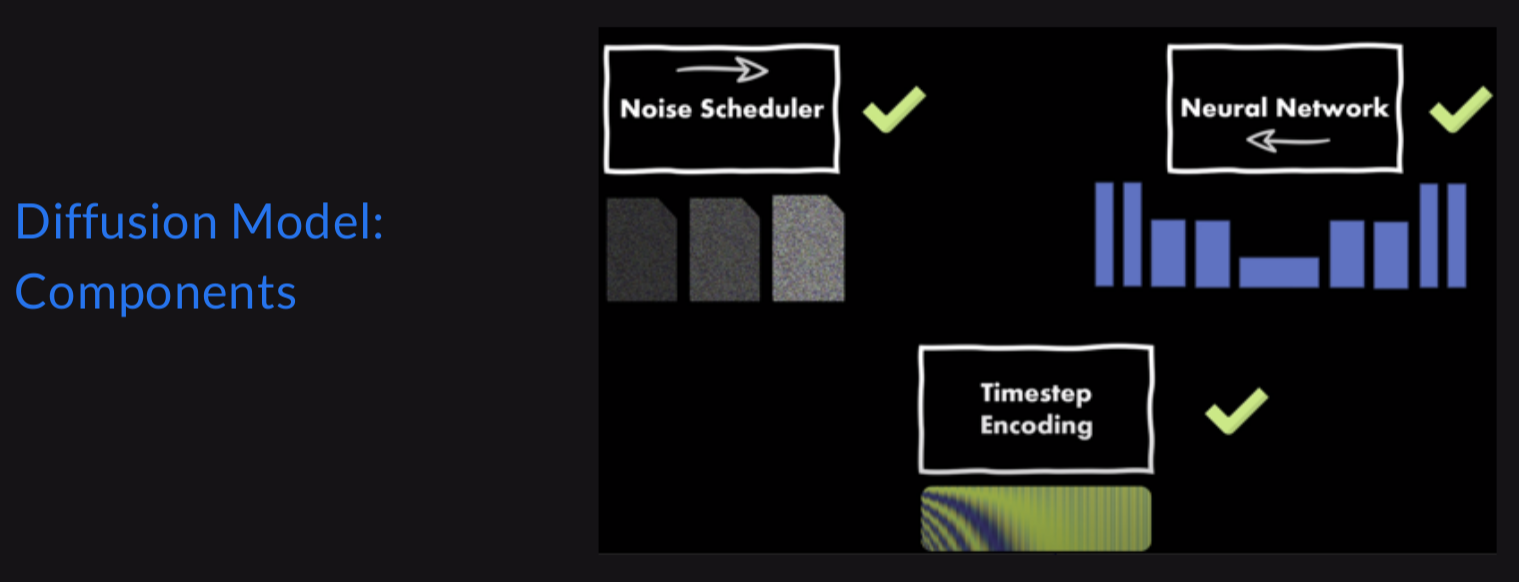
Essential elements of the ahead course of encompass:

• Gaussian noise is progressively added to the picture by the mannequin over a number of timesteps in tiny increments.
• The Markov property states that each step in a ahead course of solely depends upon the step earlier than it, making a Markov chain.
• Gaussian convergence: The information distribution converges to a Gaussian distribution after a enough variety of steps.

Listed below are the elements of the diffusion mannequin:

Implementation of the Ahead Diffusion Course of

The code on this pocket book is customized from Brian Pulfer’s DDPM implementation in his GitHub repo.

Importing obligatory libraries

# Import of libraries

import random

import imageio

import numpy as np

from argparse import ArgumentParser

from tqdm.auto import tqdm

import matplotlib.pyplot as plt

import einops

import torch

import torch.nn as nn

from torch.optim import Adam

from torch.utils.information import DataLoader

from torchvision.transforms import Compose, ToTensor, Lambda

from torchvision.datasets.mnist import MNIST, FashionMNIST

# Setting reproducibility

SEED = 0

random.seed(SEED)

np.random.seed(SEED)

torch.manual_seed(SEED)

# Definitions

STORE_PATH_MNIST = f"ddpm_model_mnist.pt"

STORE_PATH_FASHION = f"ddpm_model_fashion.pt"

Setting SEED for reproducibility

no_train = False

trend = True

batch_size = 128

n_epochs = 20

lr = 0.001

store_path = "ddpm_fashion.pt" if trend else "ddpm_mnist.pt"

Setting some parameters, no_train is ready to False. This means that we’ll practice the mannequin, and never use any pretrained mannequin. Batch_size, n_epochs, and lr are basic deep-learning parameters. We might be utilizing the Vogue MNIST dataset right here. 

Loading Knowledge

# Loading the information (changing every picture right into a tensor and normalizing between [-1, 1])

remodel = Compose([

   ToTensor(),

   Lambda(lambda x: (x - 0.5) * 2)]

)

ds_fn = FashionMNIST if trend else MNIST

dataset = ds_fn("./datasets", obtain=True, practice=True, remodel=remodel)

loader = DataLoader(dataset, batch_size, shuffle=True)

We’ll use the pytorch information loader to load our Vogue MNIST Dataset.

Ahead Diffusion Course of perform

def ahead(self, x0, t, eta=None):

       n, c, h, w = x0.form

       a_bar = self.alpha_bars[t]

       if eta is None:

           eta = torch.randn(n, c, h, w).to(self.system)

       noisy = a_bar.sqrt().reshape(n, 1, 1, 1) * x0 + (1 - a_bar).sqrt().reshape(n, 1, 1, 1) * eta

       return noisy

The above perform implements the ahead diffusion equation on to the specified step. Word: Right here, we don’t induce noise at every timestep; as a substitute, we learn the picture on the timestep straight. 

def show_forward(ddpm, loader, system):

   # Displaying the ahead course of

   for batch in loader:

       imgs = batch[0]

       show_images(imgs, "Authentic photos")

       for p.c in [0.25, 0.5, 0.75, 1]:

           show_images(

               ddpm(imgs.to(system),

                    [int(percent * ddpm.n_steps) - 1 for _ in range(len(imgs))]),

               f"DDPM Noisy photos {int(p.c * 100)}%"

           )

       break

The above code will assist us visualize the picture noise at totally different ranges: 25%, 50%, 75%, and 100%. 

Reverse Diffusion Course of

The core of steady diffusion is the reverse course of, which teaches the mannequin to piece collectively noisy photos into high-quality ones. This course of, employed for coaching and picture technology, is the other of the ahead course of.

Essential elements of the other process:

• Iterative denoising: The unique picture is progressively revealed because the mannequin progressively removes the noise.
• Noise prediction: The mannequin makes predictions concerning the noise within the present picture at every step.
• Managed technology: Extra management over the creation of photos is feasible because of the reverse course of, which allows interventions at explicit timesteps.

Additionally Learn: Unraveling the Energy of Diffusion Fashions in Trendy AI

Implementation of Reverse Diffusion Course of

def backward(self, x, t):

       # Run every picture by the community for every timestep t within the vector t.

       # The community returns its estimation of the noise that was added.

       return self.community(x, t)

Properly you might say that the reverse diffusion course of perform could be very easy, it’s as a result of in reverse diffusion the community (we are going to look into the community half quickly) predicts the quantity of noise, calculates the loss with the unique noise to study. Therefore, the code could be very easy. Under is the code for your complete DDPM – Denoise Diffusion Probabilistic Mannequin. 

The beneath code creates a Denoising Diffusion Probabilistic Mannequin (DDPM) and defines the MyDDPM PyTorch module. The ahead diffusion course of is applied by the ahead approach, which provides noise to an enter picture primarily based on a predetermined timestep. The backward method, important for the reverse diffusion course of, estimates the noise in a given noisy picture at a selected timestep utilizing a neural community. The category additionally initializes diffusion course of parameters comparable to alpha and beta schedules.

# DDPM class

class MyDDPM(nn.Module):

   def __init__(self, community, n_steps=200, min_beta=10 ** -4, max_beta=0.02, system=None, image_chw=(1, 28, 28)):

       tremendous(MyDDPM, self).__init__()

       self.n_steps = n_steps

       self.system = system

       self.image_chw = image_chw

       self.community = community.to(system)

       self.betas = torch.linspace(min_beta, max_beta, n_steps).to(

           system)  # Variety of steps is usually within the order of 1000's

       self.alphas = 1 - self.betas

       self.alpha_bars = torch.tensor([torch.prod(self.alphas[:i + 1]) for i in vary(len(self.alphas))]).to(system)

   def ahead(self, x0, t, eta=None):

       # Make enter picture extra noisy (we are able to straight skip to the specified step)

       n, c, h, w = x0.form

       a_bar = self.alpha_bars[t]

       if eta is None:

           eta = torch.randn(n, c, h, w).to(self.system)

       noisy = a_bar.sqrt().reshape(n, 1, 1, 1) * x0 + (1 - a_bar).sqrt().reshape(n, 1, 1, 1) * eta

       return noisy

   def backward(self, x, t):

       # Run every picture by the community for every timestep t within the vector t.

       # The community returns its estimation of the noise that was added.

       return self.community(x, t)

The parameters are n_steps, which tells us the variety of timesteps within the coaching course of. min_beta and max_beta point out the noise schedule, which we are going to focus on quickly.

def generate_new_images(ddpm, n_samples=16, system=None, frames_per_gif=100, gif_name="sampling.gif", c=1, h=28, w=28):

   """Given a DDPM mannequin, quite a few samples to be generated and a tool, returns some newly generated samples"""

   frame_idxs = np.linspace(0, ddpm.n_steps, frames_per_gif).astype(np.uint)

   frames = []

   with torch.no_grad():

       if system is None:

           system = ddpm.system

       # Ranging from random noise

       x = torch.randn(n_samples, c, h, w).to(system)

       for idx, t in enumerate(checklist(vary(ddpm.n_steps))[::-1]):

           # Estimating noise to be eliminated

           time_tensor = (torch.ones(n_samples, 1) * t).to(system).lengthy()

           eta_theta = ddpm.backward(x, time_tensor)

           alpha_t = ddpm.alphas[t]

           alpha_t_bar = ddpm.alpha_bars[t]

           # Partially denoising the picture

           x = (1 / alpha_t.sqrt()) * (x - (1 - alpha_t) / (1 - alpha_t_bar).sqrt() * eta_theta)

           if t > 0:

               z = torch.randn(n_samples, c, h, w).to(system)

               # Choice 1: sigma_t squared = beta_t

               beta_t = ddpm.betas[t]

               sigma_t = beta_t.sqrt()

               # Choice 2: sigma_t squared = beta_tilda_t

               # prev_alpha_t_bar = ddpm.alpha_bars[t-1] if t > 0 else ddpm.alphas[0]

               # beta_tilda_t = ((1 - prev_alpha_t_bar)/(1 - alpha_t_bar)) * beta_t

               # sigma_t = beta_tilda_t.sqrt()

               # Including some extra noise like in Langevin Dynamics trend

               x = x + sigma_t * z

           # Including frames to the GIF

           if idx in frame_idxs or t == 0:

               # Placing digits in vary [0, 255]

               normalized = x.clone()

               for i in vary(len(normalized)):

                   normalized[i] -= torch.min(normalized[i])

                   normalized[i] *= 255 / torch.max(normalized[i])

               # Reshaping batch (n, c, h, w) to be a (as a lot because it will get) sq. body

               body = einops.rearrange(normalized, "(b1 b2) c h w -> (b1 h) (b2 w) c", b1=int(n_samples ** 0.5))

               body = body.cpu().numpy().astype(np.uint8)

               # Rendering body

               frames.append(body)

   # Storing the gif

   with imageio.get_writer(gif_name, mode="I") as author:

       for idx, body in enumerate(frames):

           # Convert grayscale body to RGB

           rgb_frame = np.repeat(body, 3, axis=-1)

           author.append_data(rgb_frame)

           if idx == len(frames) - 1:

               for _ in vary(frames_per_gif // 3):

                   author.append_data(rgb_frame)

   return x

The above code is our perform for producing new photos. It creates 16 new photos. The reverse strategy of these 16 new photos is captured at every timestep, however solely 100 are taken from 200 timesteps. Then, these 100 frames are changed into GIFs to indicate the visualization of our model-generating photos. 

The above code might be generated as soon as the community is ready. Now, let’s look into the neural community.

Additionally learn: Implementing Diffusion Fashions for Artistic AI Artwork Technology

Neural Community Structure

Earlier than we glance into the structure of our neural community, which we are going to use to generate photos. We should always know that the diffusion mannequin’s parameters are shared throughout totally different timesteps. It should take away noise from photos with broadly totally different ranges of noise. Therefore, we’ve positional encoding, which encodes the timestep utilizing a sinusoidal perform to deal with this. 

Implementation of Positional Encoding

Key elements of positional encoding:

• Distinct illustration: Every timestep is given a novel vector illustration.
• Noise stage consciousness: Helps the mannequin perceive the present noise stage, permitting for acceptable denoising choices.
• Course of steering: Guides the mannequin by totally different phases of the diffusion course of.

def sinusoidal_embedding(n, d):

   # Returns the usual positional embedding

   embedding = torch.zeros(n, d)

   wk = torch.tensor([1 / 10_000 ** (2 * j / d) for j in range(d)])

   wk = wk.reshape((1, d))

   t = torch.arange(n).reshape((n, 1))

   embedding[:,::2] = torch.sin(t * wk[:,::2])

   embedding[:,1::2] = torch.cos(t * wk[:,::2])

   return embedding

Now that we’ve seen positional encoding to differentiate between timesteps, we are going to look into our Neural Community Structure. UNet is the most typical structure used within the diffusion mannequin as a result of it really works on the picture’s pixel stage. It encompasses a symmetric encoder-decoder construction with skip connections between corresponding layers. In Steady Diffusion, U-Internet predicts the noise at every denoising step. Its potential to seize and mix options at totally different scales makes it notably efficient for picture technology duties, permitting the mannequin to keep up advantageous particulars and world construction within the generated photos.

Let’s declare UNet for our steady diffusion course of. 

class MyUNet(nn.Module):

   '''

   Vanilla UNet Implementation with Timesteps Positional Ecndoing being utilized in each block along with Common enter from earlier block

   '''

   def __init__(self, n_steps=1000, time_emb_dim=100):

       tremendous(MyUNet, self).__init__()

       # Sinusoidal embedding

       self.time_embed = nn.Embedding(n_steps, time_emb_dim)

       self.time_embed.weight.information = sinusoidal_embedding(n_steps, time_emb_dim)

       self.time_embed.requires_grad_(False)

       # First half

       self.te1 = self._make_te(time_emb_dim, 1)

       self.b1 = nn.Sequential(

           MyBlock((1, 28, 28), 1, 10),

           MyBlock((10, 28, 28), 10, 10),

           MyBlock((10, 28, 28), 10, 10)

       )

       self.down1 = nn.Conv2d(10, 10, 4, 2, 1)

       self.te2 = self._make_te(time_emb_dim, 10)

       self.b2 = nn.Sequential(

           MyBlock((10, 14, 14), 10, 20),

           MyBlock((20, 14, 14), 20, 20),

           MyBlock((20, 14, 14), 20, 20)

       )

       self.down2 = nn.Conv2d(20, 20, 4, 2, 1)

       self.te3 = self._make_te(time_emb_dim, 20)

       self.b3 = nn.Sequential(

           MyBlock((20, 7, 7), 20, 40),

           MyBlock((40, 7, 7), 40, 40),

           MyBlock((40, 7, 7), 40, 40)

       )

       self.down3 = nn.Sequential(

           nn.Conv2d(40, 40, 2, 1),

           nn.SiLU(),

           nn.Conv2d(40, 40, 4, 2, 1)

       )

       # Bottleneck

       self.te_mid = self._make_te(time_emb_dim, 40)

       self.b_mid = nn.Sequential(

           MyBlock((40, 3, 3), 40, 20),

           MyBlock((20, 3, 3), 20, 20),

           MyBlock((20, 3, 3), 20, 40)

       )

       # Second half

       self.up1 = nn.Sequential(

           nn.ConvTranspose2d(40, 40, 4, 2, 1),

           nn.SiLU(),

           nn.ConvTranspose2d(40, 40, 2, 1)

       )

       self.te4 = self._make_te(time_emb_dim, 80)

       self.b4 = nn.Sequential(

           MyBlock((80, 7, 7), 80, 40),

           MyBlock((40, 7, 7), 40, 20),

           MyBlock((20, 7, 7), 20, 20)

       )

       self.up2 = nn.ConvTranspose2d(20, 20, 4, 2, 1)

       self.te5 = self._make_te(time_emb_dim, 40)

       self.b5 = nn.Sequential(

           MyBlock((40, 14, 14), 40, 20),

           MyBlock((20, 14, 14), 20, 10),

           MyBlock((10, 14, 14), 10, 10)

       )

       self.up3 = nn.ConvTranspose2d(10, 10, 4, 2, 1)

       self.te_out = self._make_te(time_emb_dim, 20)

       self.b_out = nn.Sequential(

           MyBlock((20, 28, 28), 20, 10),

           MyBlock((10, 28, 28), 10, 10),

           MyBlock((10, 28, 28), 10, 10, normalize=False)

       )

       self.conv_out = nn.Conv2d(10, 1, 3, 1, 1)

   def ahead(self, x, t):

       # x is (N, 2, 28, 28) (picture with positional embedding stacked on channel dimension)

       t = self.time_embed(t)

       n = len(x)

       out1 = self.b1(x + self.te1(t).reshape(n, -1, 1, 1))  # (N, 10, 28, 28)

       out2 = self.b2(self.down1(out1) + self.te2(t).reshape(n, -1, 1, 1))  # (N, 20, 14, 14)

       out3 = self.b3(self.down2(out2) + self.te3(t).reshape(n, -1, 1, 1))  # (N, 40, 7, 7)

       out_mid = self.b_mid(self.down3(out3) + self.te_mid(t).reshape(n, -1, 1, 1))  # (N, 40, 3, 3)

       out4 = torch.cat((out3, self.up1(out_mid)), dim=1)  # (N, 80, 7, 7)

       out4 = self.b4(out4 + self.te4(t).reshape(n, -1, 1, 1))  # (N, 20, 7, 7)

       out5 = torch.cat((out2, self.up2(out4)), dim=1)  # (N, 40, 14, 14)

       out5 = self.b5(out5 + self.te5(t).reshape(n, -1, 1, 1))  # (N, 10, 14, 14)

       out = torch.cat((out1, self.up3(out5)), dim=1)  # (N, 20, 28, 28)

       out = self.b_out(out + self.te_out(t).reshape(n, -1, 1, 1))  # (N, 1, 28, 28)

       out = self.conv_out(out)

       return out

   def _make_te(self, dim_in, dim_out):

       return nn.Sequential(

           nn.Linear(dim_in, dim_out),

           nn.SiLU(),

           nn.Linear(dim_out, dim_out)

       )

Instantiating the mannequin

# Defining mannequin

n_steps, min_beta, max_beta = 1000, 10 ** -4, 0.02  # Initially utilized by the authors

ddpm = MyDDPM(MyUNet(n_steps), n_steps=n_steps, min_beta=min_beta, max_beta=max_beta, system=system)

#Variety of parameters within the mannequin to be realized.

sum([p.numel() for p in ddpm.parameters()])

Visualization of Ahead diffusion

show_forward(ddpm, loader, system)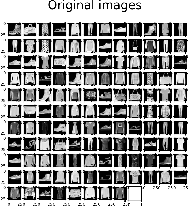

The above-mentioned photos are unique Vogue MNIST photos with none noise. Right here, we are going to take these photos and slowly inducing noise into them. 

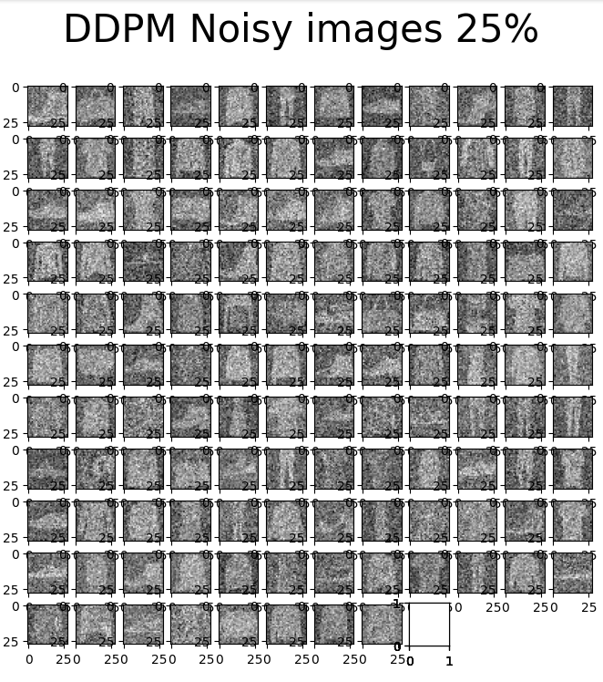
We will observe from the above-mentioned photos that there’s noise within the photos, however it’s not troublesome to acknowledge them. We add noise as per our noise schedule. The above photos include 25% of the noise as per the linear noise schedule. 

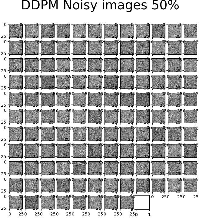
We will see that the noise is being progressively added till 100% of the picture is noise. The above picture exhibits 50% of the noise added as per noise schedule and at 50% we’re unable to recognise photos, that is thought of a disadvantage of linear noise schedule and up to date diffusion fashions use extra superior strategies to induce noise. 

Producing Photographs Earlier than Coaching

generated = generate_new_images(ddpm, gif_name="before_training.gif")
show_images(generated, "Photographs generated earlier than coaching")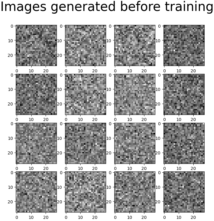

We will see that the mannequin is aware of nothing concerning the dataset and may generate solely noise. Earlier than we begin coaching our mannequin, we are going to focus on the noise schedule. 

Noise Schedule

The noise schedule is a important part in diffusion fashions. It determines how noise is added through the ahead course of and eliminated through the reverse course of. It additionally defines the speed at which data is destroyed and reconstructed, considerably impacting the mannequin’s efficiency and the standard of generated samples.

A well-designed noise schedule balances the trade-off between technology high quality and computational effectivity. Too speedy noise addition can result in data loss and poor reconstruction, whereas too sluggish a schedule may end up in unnecessarily lengthy computation occasions. Superior strategies like cosine schedules can optimize this course of, permitting for quicker sampling with out sacrificing output high quality. The noise schedule additionally influences the mannequin’s potential to seize totally different ranges of element, from coarse buildings to advantageous textures, making it a key consider attaining high-fidelity generations.

In our DDPM mannequin, we are going to use a Linear Schedule the place noise is added linearly, however there are different current developments in Steady diffusion. Now that we perceive the Noise schedule let’s practice our mannequin. 

Mannequin Coaching

In mannequin coaching, we soak up our Neural Community and practice them upon the photographs that we get from ahead diffusion; the beneath perform takes our mannequin, dataset, variety of epochs, and optimizer used. eta is the unique quantity of noise added to the picture, and eta_theta is the noise predicted by the mannequin. Upon figuring out the MSE loss, utilizing the eta and eta_theta mannequin, it learns to foretell noise current within the picture. 

def training_loop(ddpm, loader, n_epochs, optim, system, show=False, store_path="ddpm_model.pt"):

   mse = nn.MSELoss()

   best_loss = float("inf")

   n_steps = ddpm.n_steps

   for epoch in tqdm(vary(n_epochs), desc=f"Coaching progress", color="#00ff00"):

       epoch_loss = 0.0

       for step, batch in enumerate(tqdm(loader, go away=False, desc=f"Epoch {epoch + 1}/{n_epochs}", color="#005500")):

           # Loading information

           x0 = batch[0].to(system)

           n = len(x0)

           # Choosing some noise for every of the photographs within the batch, a timestep and the respective alpha_bars

           eta = torch.randn_like(x0).to(system)

           t = torch.randint(0, n_steps, (n,)).to(system)

           # Computing the noisy picture primarily based on x0 and the time-step (ahead course of)

           noisy_imgs = ddpm(x0, t, eta)

           # Getting mannequin estimation of noise primarily based on the photographs and the time-step

           eta_theta = ddpm.backward(noisy_imgs, t.reshape(n, -1))

           # Optimizing the MSE between the noise plugged and the expected noise

           loss = mse(eta_theta, eta)

           optim.zero_grad()

           loss.backward()

           optim.step()

           epoch_loss += loss.merchandise() * len(x0) / len(loader.dataset)

       # Show photos generated at this epoch

       if show:

           show_images(generate_new_images(ddpm, system=system), f"Photographs generated at epoch {epoch + 1}")

       log_string = f"Loss at epoch {epoch + 1}: {epoch_loss:.3f}"

       # Storing the mannequin

       if best_loss > epoch_loss:

           best_loss = epoch_loss

           torch.save(ddpm.state_dict(), store_path)

           log_string += " --> Finest mannequin ever (saved)"

       print(log_string)

# Coaching

# Estimate - on T4 it takes round 9 minutes to do 20 epochs

store_path = "ddpm_fashion.pt" if trend else "ddpm_mnist.pt"

if not no_train:

   training_loop(ddpm, loader, n_epochs, optim=Adam(ddpm.parameters(), lr), system=system, store_path=store_path)

An individual with fundamental pytorch and deep studying data would say that that is simply regular mannequin coaching, and sure, it’s. We now have predicted noise from our mannequin and true noise from ahead diffusion. Utilizing these two, we discover loss utilizing MSE and replace our community’s weightage to learn to predict and take away noise. 

Mannequin Testing

# Loading the skilled mannequin

best_model = MyDDPM(MyUNet(), n_steps=n_steps, system=system)

best_model.load_state_dict(torch.load(store_path, map_location=system))

best_model.eval()

print("Mannequin loaded")

print("Producing new photos")

generated = generate_new_images(

       best_model,

       n_samples=100,

       system=system,

       gif_name="trend.gif" if trend else "mnist.gif"

   )

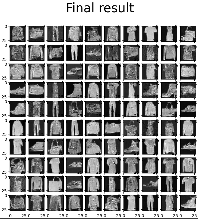
show_images(generated, "Last consequence")

We’ll attempt producing new photos (100 photos), seize the reverse course of, and make it right into a gif. 

from IPython.show import Picture

Picture(open('trend.gif' if trend else 'mnist.gif','rb').learn())

The above GIF exhibits us our community producing 100 photos; it begins from pure noise and does a reverse diffusion course of; therefore, ultimately, we get 100 newly generated photos primarily based on the training from our MNIST dataset.

Conclusion

Steady Diffusion’s spectacular picture technology capabilities consequence from the intricate interaction of those 5 key elements. The ahead and reverse processes work in tandem to study the connection between clear and noisy photos. The noise schedule optimizes the addition and elimination of noise, whereas positional encoding offers essential temporal data. Lastly, the neural community structure combines every little thing, studying to generate high-quality photos from noise or textual content descriptions.

As analysis advances, we are able to anticipate additional refinements in every part, probably resulting in extra spectacular image-generation capabilities. The way forward for AI-generated artwork and content material seems to be brighter than ever, because of the stable basis laid by Steady Diffusion and its key elements.

If you wish to grasp steady diffusion, checkout our unique GenAI Pinnacle Program immediately!

Incessantly Requested Questions