
Introduction
Understanding the importance of a phrase in a textual content is essential for analyzing and decoding massive volumes of knowledge. That is the place the time period frequency-inverse doc frequency (TF-IDF) approach in Pure Language Processing (NLP) comes into play. By overcoming the restrictions of the normal bag of phrases strategy, TF-IDF enhances textual content classification and bolsters machine studying fashions’ capacity to understand and analyze textual data successfully. This text will present you methods to construct a TF-IDF mannequin from scratch in Python and methods to compute it numerically.
Overview
- TF-IDF is a key NLP approach that enhances textual content classification by assigning significance to phrases based mostly on their frequency and rarity.
- Important phrases, together with Time period Frequency (TF), Doc Frequency (DF), and Inverse Doc Frequency (IDF), are outlined.
- The article particulars the step-by-step numerical calculation of TF-IDF scores, reminiscent of paperwork.
- A sensible information to utilizing
TfidfVectorizerfrom scikit-learn to transform textual content paperwork right into a TF-IDF matrix. - It’s utilized in engines like google, textual content classification, clustering, and summarization however doesn’t take into account phrase order or context.
Terminology: Key Phrases Utilized in TF-IDF
Earlier than diving into the calculations and code, it’s important to know the important thing phrases:
- t: time period (phrase)
- d: doc (set of phrases)
- N: rely of corpus
- corpus: the whole doc set
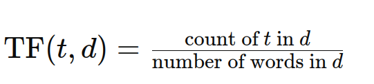
What’s Time period Frequency (TF)?
The frequency with which a time period happens in a doc is measured by time period frequency (TF). A time period’s weight in a doc is straight correlated with its frequency of incidence. The TF method is:
What’s Doc Frequency (DF)?
The importance of a doc inside a corpus is gauged by its Doc Frequency (DF). DF counts the variety of papers that include the phrase no less than as soon as, versus TF, which counts the cases of a time period in a doc. The DF method is:
DF(t)=incidence of t in paperwork
What’s Inverse Doc Frequency (IDF)?
The informativeness of a phrase is measured by its inverse doc frequency, or IDF. All phrases are given an identical weight whereas calculating TF, though IDF helps scale up unusual phrases and overwhelm widespread ones (like cease phrases). The IDF method is:
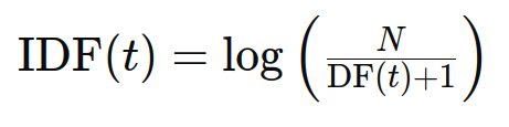
the place N is the whole variety of paperwork and DF(t) is the variety of paperwork containing the time period t.
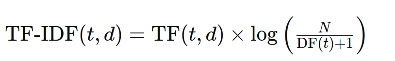
What’s TF-IDF?
TF-IDF stands for Time period Frequency-Inverse Doc Frequency, a statistical measure used to judge how necessary a phrase is to a doc in a group or corpus. It combines the significance of a time period in a doc (TF) with the time period’s rarity throughout the corpus (IDF). The method is:
Numerical Calculation of TF-IDF
Let’s break down the numerical calculation of TF-IDF for the given paperwork:
Paperwork:
- “The sky is blue.”
- “The solar is vibrant right this moment.”
- “The solar within the sky is vibrant.”
- “We will see the shining solar, the intense solar.”
Step 1: Calculate Time period Frequency (TF)
Doc 1: “The sky is blue.”
| Time period | Depend | TF |
| the | 1 | 1/4 |
| sky | 1 | 1/4 |
| is | 1 | 1/4 |
| blue | 1 | 1/4 |
Doc 2: “The solar is vibrant right this moment.”
| Time period | Depend | TF |
| the | 1 | 1/5 |
| solar | 1 | 1/5 |
| is | 1 | 1/5 |
| vibrant | 1 | 1/5 |
| right this moment | 1 | 1/5 |
Doc 3: “The solar within the sky is vibrant.”
| Time period | Depend | TF |
| the | 2 | 2/7 |
| solar | 1 | 1/7 |
| in | 1 | 1/7 |
| sky | 1 | 1/7 |
| is | 1 | 1/7 |
| vibrant | 1 | 1/7 |
Doc 4: “We will see the shining solar, the intense solar.”
| Time period | Depend | TF |
| we | 1 | 1/9 |
| can | 1 | 1/9 |
| see | 1 | 1/9 |
| the | 2 | 2/9 |
| shining | 1 | 1/9 |
| solar | 2 | 2/9 |
| vibrant | 1 | 1/9 |
Step 2: Calculate Inverse Doc Frequency (IDF)
Utilizing N=4N = 4N=4:
| Time period | DF | IDF |
| the | 4 | log(4/4+1)=log(0.8)≈−0.223 |
| sky | 2 | log(4/2+1)=log(1.333)≈0.287 |
| is | 3 | log(4/3+1)=log(1)=0 |
| blue | 1 | log(4/1+1)=log(2)≈0.693 |
| solar | 3 | log(4/3+1)=log(1)=0 |
| vibrant | 3 | log(4/3+1)=log(1)=0 |
| right this moment | 1 | log(4/1+1)=log(2)≈0.693 |
| in | 1 | log(4/1+1)=log(2)≈0.693 |
| we | 1 | log(4/1+1)=log(2)≈0.693 |
| can | 1 | log(4/1+1)=log(2)≈0.693 |
| see | 1 | log(4/1+1)=log(2)≈0.693 |
| shining | 1 | log(4/1+1)=log(2)≈0.693 |
Step 3: Calculate TF-IDF
Now, let’s calculate the TF-IDF values for every time period in every doc.
Doc 1: “The sky is blue.”
| Time period | TF | IDF | TF-IDF |
| the | 0.25 | -0.223 | 0.25 * -0.223 ≈-0.056 |
| sky | 0.25 | 0.287 | 0.25 * 0.287 ≈ 0.072 |
| is | 0.25 | 0 | 0.25 * 0 = 0 |
| blue | 0.25 | 0.693 | 0.25 * 0.693 ≈ 0.173 |
Doc 2: “The solar is vibrant right this moment.”
| Time period | TF | IDF | TF-IDF |
| the | 0.2 | -0.223 | 0.2 * -0.223 ≈ -0.045 |
| solar | 0.2 | 0 | 0.2 * 0 = 0 |
| is | 0.2 | 0 | 0.2 * 0 = 0 |
| vibrant | 0.2 | 0 | 0.2 * 0 = 0 |
| right this moment | 0.2 | 0.693 | 0.2 * 0.693 ≈0.139 |
Doc 3: “The solar within the sky is vibrant.”
| Time period | TF | IDF | TF-IDF |
| the | 0.285 | -0.223 | 0.285 * -0.223 ≈ -0.064 |
| solar | 0.142 | 0 | 0.142 * 0 = 0 |
| in | 0.142 | 0.693 | 0.142 * 0.693 ≈0.098 |
| sky | 0.142 | 0.287 | 0.142 * 0.287≈0.041 |
| is | 0.142 | 0 | 0.142 * 0 = 0 |
| vibrant | 0.142 | 0 | 0.142 * 0 = 0 |
Doc 4: “We will see the shining solar, the intense solar.”
| Time period | TF | IDF | TF-IDF |
| we | 0.111 | 0.693 | 0.111 * 0.693 ≈0.077 |
| can | 0.111 | 0.693 | 0.111 * 0.693 ≈0.077 |
| see | 0.111 | 0.693 | 0.111 * 0.693≈0.077 |
| the | 0.222 | -0.223 | 0.222 * -0.223≈-0.049 |
| shining | 0.111 | 0.693 | 0.111 * 0.693 ≈0.077 |
| solar | 0.222 | 0 | 0.222 * 0 = 0 |
| vibrant | 0.111 | 0 | 0.111 * 0 = 0 |
TF-IDF Implementation in Python Utilizing an Inbuilt Dataset
Now let’s apply the TF-IDF calculation utilizing the TfidfVectorizer from scikit-learn with an inbuilt dataset.
Step 1: Set up Essential Libraries
Guarantee you’ve scikit-learn put in:
pip set up scikit-learnStep 2: Import Libraries
import pandas as pd
from sklearn.datasets import fetch_20newsgroups
from sklearn.feature_extraction.textual content import TfidfVectorizer
Step 3: Load the Dataset
Fetch the 20 Newsgroups dataset:
newsgroups = fetch_20newsgroups(subset="prepare")Step 4: Initialize TfidfVectorizer
vectorizer = TfidfVectorizer(stop_words="english", max_features=1000)Step 5: Match and Rework the Paperwork
Convert the textual content paperwork to a TF-IDF matrix:
tfidf_matrix = vectorizer.fit_transform(newsgroups.information)Step 6: View the TF-IDF Matrix
Convert the matrix to a DataFrame for higher readability:
df_tfidf = pd.DataFrame(tfidf_matrix.toarray(), columns=vectorizer.get_feature_names_out())
df_tfidf.head()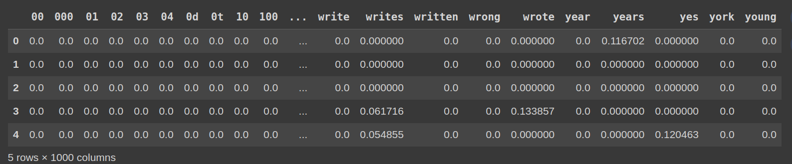
Conclusion
By utilizing the 20 Newsgroups dataset and TfidfVectorizer, you’ll be able to convert a big assortment of textual content paperwork right into a TF-IDF matrix. This matrix numerically represents the significance of every time period in every doc, facilitating varied NLP duties reminiscent of textual content classification, clustering, and extra superior textual content evaluation. The TfidfVectorizer from scikit-learn offers an environment friendly and simple technique to obtain this transformation.
Incessantly Requested Questions
Ans. A: Taking the log of IDF helps to scale down the impact of extraordinarily widespread phrases and stop the IDF values from exploding, particularly in massive corpora. It ensures that IDF values stay manageable and reduces the affect of phrases that seem very often throughout paperwork.
Ans. Sure, TF-IDF can be utilized for big datasets. Nevertheless, environment friendly implementation and sufficient computational assets are required to deal with the massive matrix computations concerned.
Ans. The TF-IDF’s limitation is that it doesn’t account for phrase order or context, treating every time period independently and thus doubtlessly lacking the nuanced that means of phrases or the connection between phrases.
Ans. TF-IDF is utilized in varied purposes, together with:
1. Search engines like google and yahoo to rank paperwork based mostly on relevance to a question
2. Textual content classification to establish essentially the most important phrases for categorizing paperwork
3. Clustering to group comparable paperwork based mostly on key phrases
4. Textual content summarization to extract necessary sentences from a doc