
The hunt for scene understanding in pc imaginative and prescient has led to many segmentation duties. Panoptic segmentation is a brand new strategy that mixes semantic and occasion segmentation into one framework.
This method identifies every pixel captured inside a picture whereas distinguishing distinct cases belonging to the identical object courses. This text will dive into the small print of panoptic segmentation, functions, and challenges.
Panoptic Segmentation
Panoptic segmentation is a reasonably attention-grabbing downside in pc imaginative and prescient today. The objective is to separate a picture into two sorts – semantic areas and occasion areas. The semantic areas are the components of the picture that belong to sure object courses, like an individual or automotive. The occasion areas are like the person folks or autos.
Not like conventional semantic segmentation, which labels pixels as belonging to particular classes like “individual” or “automotive,” panoptic segmentation goes deeper. It labels pixels with their class and distinguishes between particular person cases within the picture. This strategy goals to supply extra data in a single output, a extra detailed understanding of the scene than what conventional strategies can do.
Process Format Rationalization
Labels underneath “stuff” are steady areas with no boundaries or countable options like sky, roadways, and grass. These areas are segmented utilizing Totally Convolutional Networks (FCNs), that are good at segmenting broad background areas. The classification for distinct objects with recognizable options like folks, vehicles, or animals falls underneath the label “factor.”
These objects are segmented utilizing occasion segmentation networks, which may determine and isolate particular person cases. It will probably additionally assign a novel id to every object. This makes use of a twin labeling technique to make sure all objects within the map have semantic data and exact occasion delineation.
Introduction to the Panoptic High quality (PQ) Metric
The most recent innovation in analysis metrics is The Panoptic High quality (PQ). It was constructed to repair the issues with conventional segmentation analysis strategies. PQ is for panoptic segmentation, combining semantic and occasion segmentation by assigning a category label and an occasion ID to every pixel within the picture.
Phase Matching Course of
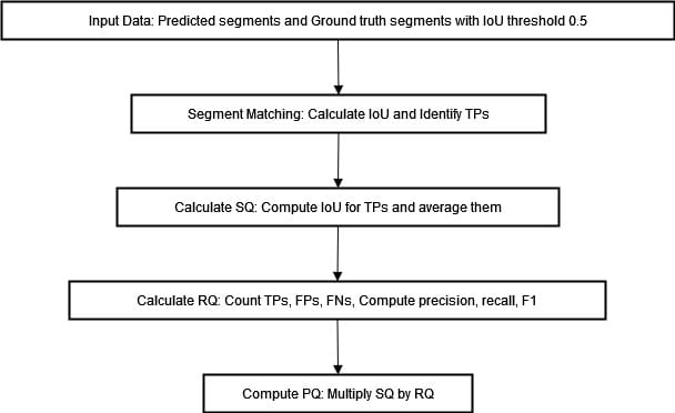
The preliminary step within the PQ metric computation is to carry out a segment-matching course of. This entails matching predicted segments with floor fact segments based mostly on their Intersection over Union (IoU) values.
A match is deemed to have occurred when the Intersection over Union (IoU) worth – a ratio that measures the overlap between predicted and floor fact segments – surpasses a predefined threshold generally set at 0.5. This may be expressed in mathematical phrases as follows:
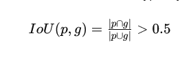
The edge as talked about above ensures that solely these segments that show substantial overlap are thought to be viable matches. Because of this, accurately segmented areas may be precisely recognized whereas mitigating false positives and negatives.
PQ Computation
Upon profitable matching of the segments, computation of the PQ metric ensues by an evaluation of segmentation high quality (SQ) and recognition high quality(RQ).
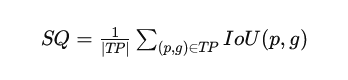
The segmentation high quality (SQ) metric assesses the typical intersection over union (IoU) of the match segments. It signifies how nicely the expected segments overlap with the bottom fact.
The popularity high quality (RQ) measures the F1 rating of the matched segments, balancing precision and recall.
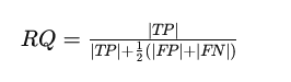
Right here, TP stands for true positives, FP for false positives, and FN for false negatives. The PQ metric is then calculated because the product of those two parts:
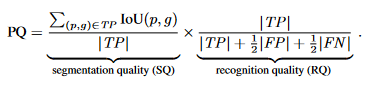
The formulation above encapsulates the parts of the PQ metric. We will visualize the method of computing PQ within the diagram under.
Benefits Over Current Metrics
The PQ metric confers a number of advantages over present metrics utilized for assessing segmentation duties. Standard metrics, equivalent to imply Intersection over Union (mIoU) or Common Precision (AP), focus solely on semantic segmentation or occasion segmentation individually, however not each.
The PQ metric presents a consolidated evaluation framework that evaluates the efficiency of panoptic segmentation fashions. This strategy proves particularly advantageous for functions the place thorough scene understanding is important. Examples embrace autonomous driving and robotics. Object classification and particular person occasion identification assume pivotal significance in such eventualities.
Machine Efficiency on Panoptic Segmentation
State-of-the-art Panoptic Segmentation strategies mix the newest occasion and semantic segmentation strategies by a heuristic merging course of.
The strategy begins by producing separate, non-overlapping predictions for issues and stuff utilizing the newest strategies. These are then mixed to get a panoptic segmentation of the picture.
In instances the place there’s a battle between factor and stuff prediction, our heuristic strategy favors the factor class. This ends in constant efficiency for factor courses (PQTh) and barely worse efficiency for stuff courses (PQSt).
Throughout numerous datasets, there are notable disparities when evaluating machine efficiency with human consistency. On Cityscapes, ADE20k, and Mapillary Vistas, people ship superior outcomes in comparison with machines.
The hole is particularly evident within the Recognition High quality (RQ) metric, which measures F1 rating accuracy. On the ADE20k dataset, people get an RQ of 78.6%, and machines get round 43.2%.
The Segmentation High quality (SQ) metric, which measures the typical IoU of matched segments, exhibits a smaller hole between people and machine. Machines are getting higher at segmentation however wrestle to acknowledge and classify objects and areas.
| Dataset | Metric | Human | Machine |
|---|---|---|---|
| Cityscapes | PQ | 69.6 | 61.2 |
| SQ | 84.1 | 80.9 | |
| RQ | 82.0 | 74.4 | |
| ADE20k | PQ | 67.6 | 35.6 |
| SQ | 85.7 | 74.4 | |
| RQ | 78.6 | 43.2 | |
| Vistas | PQ | 57.7 | 38.3 |
| SQ | 79.7 | 73.6 | |
| RQ | 71.6 | 47.7 |
The desk above exhibits the human vs machine efficiency throughout completely different datasets and metrics. The findings underscore vital areas the place enhancements are crucial for machines’ Panoptic Segmentation algorithms.
Panoptic Segmentation Utilizing DETR
we show how you can discover the panoptic segmentation capabilities of DETR. The prediction happens in a number of steps:
Deliver this venture to life
Putting in the Required Packages and Importing the Needed Libraries
The code under is a set of Python imports and configurations generally utilized in pc imaginative and prescient and image-processing duties.
from PIL import Picture
import requests
import io
import math
import matplotlib.pyplot as plt
%config InlineBackend.figure_format="retina"

import torch
from torch import nn
from torchvision.fashions import resnet50
import torchvision.transforms as T
import numpy
torch.set_grad_enabled(False);
Set up the COCO 2018 Panoptic Segmentation Process API
The next command installs the COCO 2018 Panoptic Segmentation Process API. This API is used to work with the COCO dataset, a large-scale object detection, segmentation, and captioning dataset.
pip set up git+https://github.com/cocodataset/panopticapi.git
Import the COCO 2018 Panoptic Segmentation Process API and its Utility Capabilities
The code under imports the COCO 2018 Panoptic Segmentation Process API and its utility features id2rgb and rgb2id.
id2rgb takes a panoptic segmentation map that makes use of ID numbers for every pixel and converts it into an RGB picture. The enter is a 2D array of integers that characterize class IDs. The output is a 3D array of integers the place every integer is the RGB coloration of the corresponding pixel. It’s changing from a map that exhibits what object or class every pixel represents to a picture the place we see the precise colours.
The rgb2id operate converts a panoptic segmentation map from its RGB illustration to an ID illustration.
import panopticapi
from panopticapi.utils import id2rgb, rgb2id
Beginning Level for Working with COCO Dataset and API
Within the code under, the CLASSES checklist has all of the names of the completely different objects within the COCO dataset. The coco2d2 dictionary converts the category IDs within the COCO dataset to a unique numbering scheme utilized by the Detectron2 library. The rework is a PyTorch library that prepares photographs earlier than they go right into a mannequin. It resizes to 800×800, turns right into a tensor variable, and normalizes the pixel values utilizing the imply and normal deviation of the ImageNet dataset.
# These are the COCO courses
CLASSES = [
    'N/A', 'person', 'bicycle', 'car', 'motorcycle', 'airplane', 'bus',
    'train', 'truck', 'boat', 'traffic light', 'fire hydrant', 'N/A',
    'stop sign', 'parking meter', 'bench', 'bird', 'cat', 'dog', 'horse',
    'sheep', 'cow', 'elephant', 'bear', 'zebra', 'giraffe', 'N/A', 'backpack',
    'umbrella', 'N/A', 'N/A', 'handbag', 'tie', 'suitcase', 'frisbee', 'skis',
    'snowboard', 'sports ball', 'kite', 'baseball bat', 'baseball glove',
    'skateboard', 'surfboard', 'tennis racket', 'bottle', 'N/A', 'wine glass',
    'cup', 'fork', 'knife', 'spoon', 'bowl', 'banana', 'apple', 'sandwich',
    'orange', 'broccoli', 'carrot', 'hot dog', 'pizza', 'donut', 'cake',
    'chair', 'couch', 'potted plant', 'bed', 'N/A', 'dining table', 'N/A',
    'N/A', 'toilet', 'N/A', 'tv', 'laptop', 'mouse', 'remote', 'keyboard',
    'cell phone', 'microwave', 'oven', 'toaster', 'sink', 'refrigerator', 'N/A',
    'book', 'clock', 'vase', 'scissors', 'teddy bear', 'hair drier',
    'toothbrush'
]

# Detectron2 makes use of a unique numbering scheme, we construct a conversion desk
coco2d2 = {}
depend = 0
for i, c in enumerate(CLASSES):
  if c != "N/A":
    coco2d2[i] = depend
    depend+=1

# normal PyTorch mean-std enter picture normalization
rework = T.Compose([
    T.Resize(800),
    T.ToTensor(),
    T.Normalize([0.485, 0.456, 0.406], [0.229, 0.224, 0.225])
])
Load the DETR Mannequin for Panoptic Segmentation
The code under hundreds the DETR mannequin for panoptic segmentation from the Fb Analysis GitHub repository utilizing the PyTorch Hub API. Right here is an outline of the code:
mannequin, postprocessor = torch.hub.load('facebookresearch/detr', 'detr_resnet101_panoptic', pretrained=True, return_postprocessor=True, num_classes=250)
mannequin.eval();
Be aware: The picture used right here is taken from that supply
Obtain and Open the Picture
The code under downloads and opens a picture from the COCO dataset utilizing the Pillow library.
url = "http://photographs.cocodataset.org/val2017/000000281759.jpg"
im = Picture.open(requests.get(url, stream=True).uncooked)- The
requests.get()operate sends an HTTP GET request to the URL and retrieves the picture knowledge. Thestream=Trueargument specifies that the response ought to be streamed somewhat than downloaded concurrently. - The
uncookedattribute of the response object is used to entry the uncooked picture knowledge. - The
Picture.open()operate from the Pillow library is used to open the uncooked picture knowledge and create a brand newPictureobject. ThePictureobject can then carry out numerous picture processing and manipulation duties.
Run the Prediction
The code img = rework(im).unsqueeze(0) is used to preprocess a picture utilizing a PyTorch rework and convert it to a tensor. The im variable incorporates the picture knowledge as a Pillow Picture object.
# mean-std normalize the enter picture (batch-size: 1)
img = rework(im).unsqueeze(0)
out = mannequin(img)
Plot the Predicted Segmentation Masks
The next code is expounded to plotting the expected segmentation masks for objects detected in a picture utilizing the DETR mannequin for panoptic segmentation. Right here is an outline of the code.
# compute the scores, excluding the "no-object" class (the final one)
scores = out["pred_logits"].softmax(-1)[..., :-1].max(-1)[0]
# threshold the boldness
hold = scores > 0.85

# Plot all of the remaining masks
ncols = 5
fig, axs = plt.subplots(ncols=ncols, nrows=math.ceil(hold.sum().merchandise() / ncols), figsize=(18, 10))
for line in axs:
    for a in line:
        a.axis('off')
for i, masks in enumerate(out["pred_masks"][keep]):
    ax = axs[i // ncols, i % ncols]
    ax.imshow(masks, cmap="cividis")
    ax.axis('off')
fig.tight_layout()
This code first calculates the scores for the expected masks, not together with the no-object class. Then, it units a threshold solely to maintain masks that scored larger than 0. 85 confidence. The remaining masks are plotted out in a grid with 5 columns, and the variety of rows is figured based mostly on what number of masks met the brink. The out variable handed in is assumed to be a dictionary with the expected masks and logit values.
DETR’s Postprocessor
# the post-processor expects as enter the goal measurement of the predictions (which we set right here to the picture measurement)
end result = postprocessor(out, torch.as_tensor(img.form[-2:]).unsqueeze(0))[0]
The above code takes the output out and runs it by a post-processor, producing a end result. It passes the picture measurement into the postprocessor operate, which takes the supposed prediction measurement as enter and spits out a processed output. The end result variable incorporates the processed output of the post-processor utilized to the enter picture.
Visualization
The code under imports the itertools and seaborn libraries and creates a coloration palette utilizing itertools.cycle and seaborn.color_palette(). It then opens a special-format PNG file and retrieves the IDs corresponding to every masks. Lastly, it colours every masks individually utilizing the colour palette and shows the ensuing picture utilizing matplotlib. We will do a easy visualization of the end result
import itertools
import seaborn as sns
palette = itertools.cycle(sns.color_palette())

# The segmentation is saved in a special-format png
panoptic_seg = Picture.open(io.BytesIO(end result['png_string']))
panoptic_seg = numpy.array(panoptic_seg, dtype=numpy.uint8).copy()
# We retrieve the ids corresponding to every masks
panoptic_seg_id = rgb2id(panoptic_seg)

# Lastly we coloration every masks individually
panoptic_seg[:, :, :] = 0
for id in vary(panoptic_seg_id.max() + 1):
  panoptic_seg[panoptic_seg_id == id] = numpy.asarray(subsequent(palette)) * 255
plt.determine(figsize=(15,15))
plt.imshow(panoptic_seg)
plt.axis('off')
plt.present()
Output:

Panoptic Segmentation with Detectron2
On this part, we show how you can acquire a better-looking visualization by leveraging Detectron2’s plotting utilities.
Import Libraries
The code under installs detectron2 from its GitHub repository. The Visualizer class from the utils module of detectron2 is imported to facilitate environment friendly visualization of detection outcomes. The MetadataCatalog from the info module of detectron2 is imported to entry metadata pertaining to datasets.
# Set up detectron2
pip set up 'git+https://github.com/facebookresearch/detectron2.git'
from copy import deepcopy
import io
import numpy as np
import torch
from PIL import Picture
import matplotlib.pyplot as plt
from detectron2.knowledge import MetadataCatalog
from detectron2.utils.visualizer import Visualizer
Visualizing Panoptic Segmentation Predictions with DETR and Detectron2
This code extracts and processes segmentation knowledge from DETR’s predictions, adjusting class IDs to match detectron2. It defines the rgb2id operate, copies section data, reads the panoptic end result from a PNG picture, and converts it into an ID map utilizing numpy and torch. Class IDs are then transformed to align with detectron2’s COCO format earlier than visualizing the outcomes utilizing detectron2’s Visualizer.
# Outline the rgb2id operate
def rgb2id(coloration):
if isinstance(coloration, np.ndarray) and len(coloration.form) == 3:
coloration = coloration.astype(np.int32)
return coloration[:, :, 0] + 256 * coloration[:, :, 1] + 256 * 256 * coloration[:, :, 2]
return coloration
# We extract the segments data and the panoptic end result from DETR's prediction
segments_info = deepcopy(end result["segments_info"])
# Panoptic predictions are saved in a particular format png
panoptic_seg = Picture.open(io.BytesIO(end result['png_string']))
final_w, final_h = panoptic_seg.measurement
# We convert the png right into a section id map
panoptic_seg = np.array(panoptic_seg, dtype=np.uint8)
panoptic_seg = torch.from_numpy(rgb2id(panoptic_seg))
# Detectron2 makes use of a unique numbering of coco courses, right here we convert the category ids accordingly
meta = MetadataCatalog.get("coco_2017_val_panoptic_separated")
for i in vary(len(segments_info)):
c = segments_info[i]["category_id"]
segments_info[i]["category_id"] = meta.thing_dataset_id_to_contiguous_id[c] if segments_info[i]["isthing"] else meta.stuff_dataset_id_to_contiguous_id[c]
# Lastly we visualize the prediction
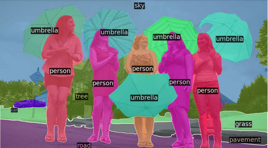
v = Visualizer(np.array(im.copy().resize((final_w, final_h)))[:, :, ::-1], meta, scale=1.0)
v._default_font_size = 20
v = v.draw_panoptic_seg_predictions(panoptic_seg, segments_info, area_threshold=0)
# Show the picture utilizing matplotlib
result_img = v.get_image()
plt.determine(figsize=(12, 8))
plt.imshow(result_img)
plt.axis('off') # Flip off axis
plt.present()Output:
Conclusion
Panoptic segmentation represents a notable leap ahead within the pc imaginative and prescient subject by unifying semantic and occasion segmentation underneath a consolidated framework. This strategy affords an in depth understanding of scenes by pixel labeling and differentiation between numerous cases of comparable object courses.
Panoptic High quality (PQ) metrics assist to judge the effectiveness of panoptic fashions whereas figuring out areas for enchancment. Whereas progress has been made, machine efficiency falls quick in comparison with human consistency.
Integrating DETR and Detectron2 highlights how additional developments may be leveraged in the direction of autonomous driving or robotics functions.