Information on Finetuning Llama 3 for Sequence Classification

Introduction

Giant Language Fashions are recognized for his or her text-generation capabilities. They’re educated with tens of millions of tokens throughout the pre-training interval. This can assist the massive language fashions perceive English textual content and generate significant full tokens throughout the era interval. One of many different frequent duties in Pure Language Processing is the Sequence Classification Process. On this, we classify the given sequence into totally different classes. This may be naively executed with Giant Language Fashions by Immediate Engineering. However this would possibly solely typically work. As a substitute, we will tweak the Giant Language Mannequin to output a set of chances for every class for a given enter. This information will present easy methods to practice such LLM and work with the finetune Llama 3 mannequin.

Studying Targets

• Perceive the fundamentals of Giant Language Fashions and their functions
• Study to finetune Llama 3 mannequin for sequence classification duties
• Discover important libraries for working with LLMs in HuggingFace
• Acquire expertise in loading and preprocessing datasets for LLM coaching
• Customise coaching processes utilizing class weights and a customized coach class

This text was printed as part of the Information Science Blogathon.

For this information, we will probably be working in Kaggle. Step one could be to obtain the required libraries that we’ll require to finetune Llama 3 for Sequence Classification. Allow us to run the code under:

!pip set up -q transformers speed up trl bitsandbytes datasets consider huggingface-cli 
!pip set up -q peft scikit-learn

Obtain Libraries

We begin by downloading the next libraries:

• Transformers: It is a library from HuggingFace, which we will use to obtain, create functions with, and fine-tune Deep Studying fashions, together with giant language fashions.
• Speed up: That is once more a library from HuggingFace that accelerates the inference velocity of the massive language fashions being run on the GPU.
• Trl: It’s a Python Package deal from HuggingFace, which we will use to fine-tune the Deep Studying Fashions accessible on the HuggingFace hub. With this TRL library, we will even fine-tune the massive language fashions.
• bitsandbytes: LLMs are very excessive in reminiscence, so we will instantly work with them in Low RAM GPUs. We quantize the Giant Language Fashions to a decrease precision so we will match them within the GPU, and for this, we require the bitsandbytes library.
• Datasets: It is a Python library from HuggingFace, with which we will obtain varied open-source datasets belonging to totally different Deep Studying and Machine Studying Classes, together with Picture Classification, Textual content Technology, Textual content Summarization, and extra.
• Consider: We are going to use this library to judge our mannequin earlier than and after coaching.
• Huggingface-cli: That is required as a result of we should log in to HuggingFace to work with the Llama3 mannequin.
• peft: With the GPU we’re working with, it’s unimaginable to coach all of the parameters of the massive language fashions. As a substitute, we will solely practice a subset of those parameters, which might be executed utilizing the peft library.
• Scikit-learn: This library incorporates many various machine studying and deep studying instruments. We are going to use this library for the error metrics to check the Giant Language Mannequin earlier than and after coaching.

After that, strive logging in to the HuggingFace hub. For this, we’ll work with the huggingface-cli instrument. The code for this may be seen under:

!huggingface-cli login --token $YOUR_HF_TOKEN

Code Rationalization

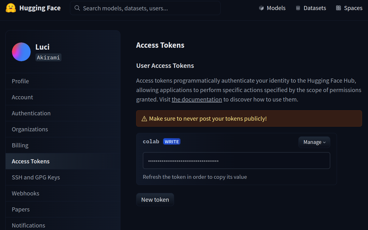
Right here, we name the login choice for the huggingface-cli with the extra – token choice. Right here we offer our HuggingFace token to log into the HuggingFace. To get the HuggingFace token, go to this hyperlink. As proven within the pic under, you possibly can create an entry token by clicking on New Token or utilizing an current token. Simply copy that token and paste it within the place YOUR_HF_TOKEN.

Let’s Load the Dataset

Subsequent, we load the dataset for coaching. For this, we work with the under code:

from datasets import load_dataset

dataset = load_dataset("ag_news")

• We begin by importing the load_dataset perform from the datasets library
• Then we name the load_dataset perform with the dataset title “ag_news”

Operating this can obtain the ag_news dataset to the dataset variable. The ag_news dataset appears to be like just like the under pic:

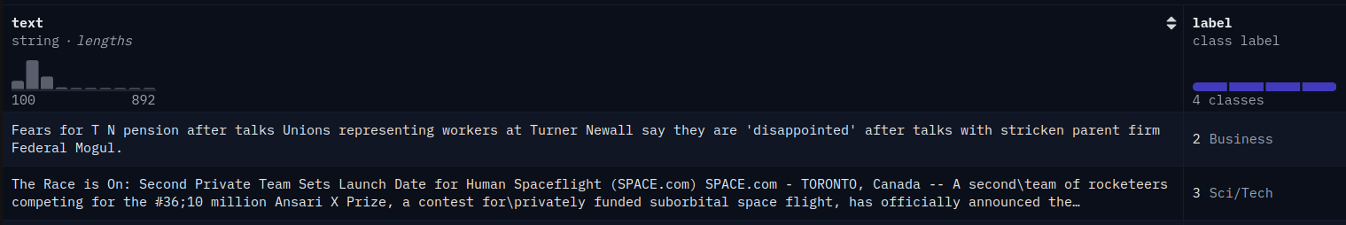
It’s a information classification dataset. The information is classed into totally different classes, reminiscent of world, sports activities, enterprise, and sci/tech. Now, allow us to see if the examples for every class are represented in equal numbers or if there may be any class imbalance.

import pandas as pd

df = pd.DataFrame(dataset['train'])

df.label.value_counts(normalize=True)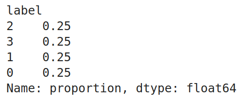

Code Rationalization

• Right here, we begin by importing the pandas library
• The ag_news dataset incorporates each the coaching set and a take a look at set. And the dataset variable of sort DatasetDict. For ease of use, we convert it into pandas DataFrame
• Then we name the value_counts() perform on the “label” column of the dataframe with normalize set to True

Operating this code produced the next output. We will test that each one 4 labels have an equal proportion, which means that every class has an equal variety of examples within the dataset. The dataset is large, so we solely want part of it. So, we pattern some information from this dataframe with the next code:

# Splitting the dataframe into 4 separate dataframes primarily based on the labels
label_1_df = df[df['label'] == 0]
label_2_df = df[df['label'] == 1]
label_3_df = df[df['label'] == 2]
label_4_df = df[df['label'] == 3]

# Shuffle every label dataframe
label_1_df = label_1_df.pattern(frac=1).reset_index(drop=True)
label_2_df = label_2_df.pattern(frac=1).reset_index(drop=True)
label_3_df = label_3_df.pattern(frac=1).reset_index(drop=True)
label_4_df = label_4_df.pattern(frac=1).reset_index(drop=True)

# Splitting every label dataframe into practice, take a look at, and validation units
label_1_train = label_1_df.iloc[:2000]
label_1_test = label_1_df.iloc[2000:2500]
label_1_val = label_1_df.iloc[2500:3000]

label_2_train = label_2_df.iloc[:2000]
label_2_test = label_2_df.iloc[2000:2500]
label_2_val = label_2_df.iloc[2500:3000]

label_3_train = label_3_df.iloc[:2000]
label_3_test = label_3_df.iloc[2000:2500]
label_3_val = label_3_df.iloc[2500:3000]

label_4_train = label_4_df.iloc[:2000]
label_4_test = label_4_df.iloc[2000:2500]
label_4_val = label_4_df.iloc[2500:3000]

# Concatenating the splits again collectively
train_df = pd.concat([label_1_train, label_2_train, label_3_train, label_4_train])
test_df = pd.concat([label_1_test, label_2_test, label_3_test, label_4_test])
val_df = pd.concat([label_1_val, label_2_val, label_3_val, label_4_val])

# Shuffle the dataframes to make sure randomness
train_df = train_df.pattern(frac=1).reset_index(drop=True)
test_df = test_df.pattern(frac=1).reset_index(drop=True)
val_df = val_df.pattern(frac=1).reset_index(drop=True)

• Our information incorporates 4 labels. So we create 4 dataframes the place every dataframe consists of a single label
• Then, we shuffle every of those labels by calling the pattern perform on them
• Then we cut up every of those label dataframes into 3 splits referred to as the practice, take a look at, and legitimate dataframes. For practice, we offer 2000 labels, and for testing and validation, we offer 500 every
• Now, we concat the coaching dataframes of all of the labels right into a single coaching dataframe by the pd.concat() perform
• We do the identical factor even for the take a look at and validation dataframes
• Lastly, we shuffle the train_df, test_df, and valid_df yet one more time to make sure randomness in them

Checking the Worth Counts

For affirmation, allow us to test the worth counts of every label within the coaching dataframe. The code for this will probably be:

train_df.label.value_counts()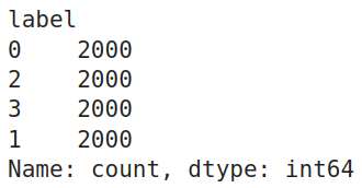

Pandas DataFrames to DatasetDict

So, we will test that the coaching dataframe has equal examples for every of the 4 labels. Earlier than sending them to coaching, we have to convert these Pandas DataFrames to DatasetDict, which the HuggingFace coaching library accepts. For this, we work with the next code:

from datasets import DatasetDict, Dataset

# Changing pandas DataFrames into Hugging Face Dataset objects:
dataset_train = Dataset.from_pandas(train_df)
dataset_val = Dataset.from_pandas(val_df)
dataset_test = Dataset.from_pandas(test_df)

# Mix them right into a single DatasetDict
dataset = DatasetDict({
    'practice': dataset_train,
    'val': dataset_val,
    'take a look at': dataset_test
})
dataset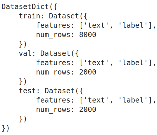

Code Rationalization

• First, we import the DatasetDict class from the datasets library
• Then we convert every of the train_df, test_df, and val_df from Pandas DataFrames to the HuggingFace Dataset sort
• Lastly, we mix all of the practice, take a look at, and val HuggingFace Dataset, create the ultimate DatasetDict sort variable, and retailer it within the dataset variable

We will see from the output that the DatasetDict incorporates 3 Datasets, that are the practice, take a look at, and validation datasets. The place every of those datasets incorporates solely 2 columns: one is textual content, and the opposite is the label.

Right here, in our dataset, the proportion of every class is similar. In sensible instances, this would possibly solely typically be true. So when the lessons are imbalanced, we have to take correct measures so the LLM doesn’t give extra significance to the label containing extra examples. For this, we calculate the category weights.

Class weights inform us how a lot significance we should give to every class; the extra class weights there are, the extra significance there may be to the category. If we now have an imbalanced dataset, we might present extra class weight to the label, having fewer examples, thus giving extra significance to it. To get these class weights, we will take the inverse of the proportion of sophistication labels (worth counts) of the dataset. The code for this will probably be:

import torch

class_weights=(1/train_df.label.value_counts(normalize=True).sort_index()).tolist()
class_weights=torch.tensor(class_weights)
class_weights=class_weights/class_weights.sum()
class_weights

Code Rationalization

• So, we begin by taking the values of the inverse of worth counts of the category labels
• Then, we convert these from a listing sort to a torch tensor sort
• We then normalize the class_weights by dividing them by the sum of class_weights

We will see from the output that the category weights are equal for all of the lessons; it is because all of the lessons have the identical variety of examples.

Additionally learn: 3 Methods to Use Llama 3 [Explained with Steps]

Mannequin Loading -Quantization

On this part, we’ll obtain and put together the mannequin for the coaching. The primary is to obtain the mannequin. We can’t work with the complete mannequin as a result of we’re coping with a small GPU; therefore, we’ll quantify it. The code for this will probably be:

from transformers import BitsAndBytesConfig, AutoModelForSequenceClassification

quantization_config = BitsAndBytesConfig(
    load_in_4bit = True, 
    bnb_4bit_quant_type="nf4",
    bnb_4bit_use_double_quant = True, 
    bnb_4bit_compute_dtype = torch.bfloat16 
)

model_name = "meta-llama/Meta-Llama-3-8B"

mannequin = AutoModelForSequenceClassification.from_pretrained(
    model_name,
    quantization_config=quantization_config,
    num_labels=4,
    device_map='auto'
)

Code Rationalization

• We import the BitsAndBytesConfig and the AutoModelForSequenceClassification lessons from the transformers library.
• We should outline a quantization config to create a quantization for the mannequin. For this, we’ll create an occasion of BitsAndBytesConfig and provides it totally different quantization parameters.
• load_in_4bit: That is set to True, which tells that we want to quantize the mannequin to a 4-bit precision
• bnb_4bit_quant_type: That is the kind of quantization we want to work with, and we will probably be going with Regular Float, aka NF4, which is the really helpful one
• bnb_4bit_compute_dtype: That is the info sort wherein the GPU computations will probably be carried out. This can often be both torch.float32 / torch.float16 / torch.bfloat16, in our instance, primarily based on the GPU, we go together with torch.bfloat16
• bnb_4bit_use_double_quant: When set to True, it’ll additional cut back the reminiscence footprint by quantizing the quantization constants
• Subsequent, we offer the mannequin title that we’ll finetune to the model_name variable, which right here is Meta’s newly launched Llama 3 8B
• Then, we create an occasion of the AutoModelForSequenceClassification class and provides it the mannequin title and the quantization config
• We additionally used one other variable referred to as the num_labels and set it to 4. What AutoModelForSequenceClassification does is take away the final layer of the Llama 3 LLM and exchange it with a linear layer
• We’re setting the output of this linear layer to 4; it is because there are 4 class labels in our dataset
• Lastly, we set the device_map to “auto,” so the mannequin will get loaded to the GPU

So operating the above will obtain the Llama 3 8B Giant Language Mannequin from the HuggingFace hub, quantize it primarily based on the quantization_config that we now have supplied to it, after which exchange the output head of the LLM with a linear head with 4 neurons for the output and pushed the mannequin to the GPU. Subsequent, we’ll create a LoRA config for the mannequin to coach solely a subset of parameters. The code for this will probably be:

LoRA Configuration

from peft import LoraConfig, prepare_model_for_kbit_training, get_peft_model

lora_config = LoraConfig(
    r = 16, 
    lora_alpha = 8,
    target_modules = ['q_proj', 'k_proj', 'v_proj', 'o_proj'],
    lora_dropout = 0.05, 
    bias="none",
    task_type="SEQ_CLS"
)

mannequin = prepare_model_for_kbit_training(mannequin)
mannequin = get_peft_model(mannequin, lora_config)

Code Rationalization

• We begin by importing LoraConfig, prepare_model_for_kbit_training, and get_peft_model from peft library
• Then, we instantiate a LoraConfig class and provides it totally different parameters, which embody
• r: This defines the rank of the matrix of parameters that we’ll be coaching. We now have set this to 16
• lora_alpha: It is a hyperparameter for the LoRA-based coaching. That is often set to half of the worth of r
• target_modules: It is a listing the place we specify the place we ought to be including the LoRA-based coaching. For this, we select all the eye layers, just like the Okay, Q, V, and the Output Projections
• lora_dropout: This we set to 0.05, which is able to randomly drop the neurons in order that overfitting doesn’t occur
• bias: If set to true, then even the bias time period will probably be added together with the weights for coaching
• task_type: As a result of we’re coaching for a classification dataset and have added the classification layer to the LLM, we will probably be conserving this “SEQ_CLS”
• Then, we name the prepare_model_for_kbit_training() perform, to which we give the mannequin. This perform preprocess the quantized mannequin for coaching
• Lastly, we name the get_peft_model() perform by giving it each the mannequin and the LoraConfig

Operating this, the get_peft_model will take the mannequin and put together it for coaching with a PEFT technique, just like the LoRA on this case, by wrapping the mannequin and the LoRA Configuration.

Mannequin Testing – Pre Coaching

On this part, we’ll take a look at the Llama 3 mannequin on the take a look at information earlier than the mannequin has been educated. To do that, we’ll first obtain the tokenizer. The code for this will probably be:

from transformers import AutoTokenizer

model_name = "meta-llama/Meta-Llama-3-8B"
tokenizer = AutoTokenizer.from_pretrained(model_name, add_prefix_space=True)

tokenizer.pad_token_id = tokenizer.eos_token_id
tokenizer.pad_token = tokenizer.eos_token

Code Rationalization

• Right here, we import the AutoTokenizer class from the transformers library
• We instantiate a tokenizer by calling the from_pretrained() perform of the AutoTokenizer class and passing it the mannequin title
• We then set the pad_token of the tokenizer to the eos_token, and the identical goes for the pad_token_id

mannequin.config.pad_token_id = tokenizer.pad_token_id
mannequin.config.use_cache = False
mannequin.config.pretraining_tp = 1

Subsequent, we even edit the mannequin configuration by setting the pad token ID of the mannequin to the pad token ID of the tokenizer and never utilizing the cache. Now, we’ll give our take a look at information to the mannequin and accumulate the outputs:

sentences = test_df.textual content.tolist()

batch_size = 32  

all_outputs = []

for i in vary(0, len(sentences), batch_size):
    batch_sentences = sentences[i:i + batch_size]

    inputs = tokenizer(batch_sentences, return_tensors="pt", 
    padding=True, truncation=True, max_length=512)

    inputs = {okay: v.to('cuda' if torch.cuda.is_available() else 'cpu') for okay, v in inputs.objects()}

    with torch.no_grad():
        outputs = mannequin(**inputs)
        all_outputs.append(outputs['logits'])
        
final_outputs = torch.cat(all_outputs, dim=0)
test_df['predictions']=final_outputs.argmax(axis=1).cpu().numpy()

Code Rationalization

• First, we convert the weather within the textual content column of the take a look at DataFrame into a listing of sentences and retailer them within the variable sentences.
• Then, we outline a batch measurement to signify the mannequin’s inputs in a batch; right here, we set this measurement to 32.
• We then create an empty listing of all_outputs to retailer the outputs that the mannequin will generate
• We begin iterating by the sentence variable with the step measurement set to the batch measurement we now have outlined.
• So, in every iteration, we tokenize the enter sentences in batches.
• Then, we transfer these tokenized sentences to the system on which we run the mannequin, both a GPU or CPU.
• Lastly, we carry out the mannequin inference by passing the inputs to the mannequin and appending the output logits to the all_outputs listing. We then concatenate all these outputs to kind a remaining output tensor.

Operating this code will retailer the mannequin leads to a variable. We are going to add these predictions to the take a look at DataFrame in a brand new column. We take the argmax of every output; this provides us the label that has the best chance for every output within the final_outputs listing. Now, we have to consider the output generated by the LLM, which we will do by the code under:

from sklearn.metrics import accuracy_score, confusion_matrix
from sklearn.metrics import balanced_accuracy_score, classification_report

def get_metrics_result(test_df):
    y_test = test_df.label
    y_pred = test_df.predictions

    print("Classification Report:")
    print(classification_report(y_test, y_pred))

    print("Balanced Accuracy Rating:", balanced_accuracy_score(y_test, y_pred))
    print("Accuracy Rating:", accuracy_score(y_test, y_pred))

get_metrics_result(test_df)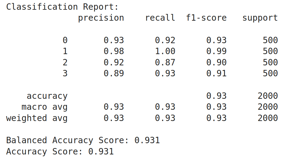

Code Rationalization

• We begin by importing the accuracy_score, balanced_accuracy_score, and classification_report from the sklearn library.
• Then we outline a perform referred to as get_metrics_result(), which takes in a dataframe and outputs the outcomes.
• On this perform, we first begin by storing the predictions and precise labels in a variable.
• Then, we give these precise and predicted values to the classification report, accuracy_score, and balance_accuracy_score, and print them.
• The balance_accuracy_score is helpful when coping with imbalanced information.

Operating that has produced the next outcomes. We will see that we get an accuracy of 0.23, which may be very low. The mannequin’s precision, recall, and f1-score are very low, too; they don’t even attain a share above 50%. Testing them after coaching the mannequin will give us an understanding of how nicely it’s educated.

Earlier than we begin coaching, we have to preprocess the info earlier than sending it to the mannequin. For this, we work with the next code:

def data_preprocesing(row):
    return tokenizer(row['text'], truncation=True, max_length=512)

tokenized_data = dataset.map(data_preprocesing, batched=True, 
remove_columns=['text'])
tokenized_data.set_format("torch")

Code Rationalization

• We outline a perform referred to as data_preprocessing(), which expects a row of information
• Inside it, we go the textual content content material of that row to the tokenizer with truncation set to true and max size set to 512 tokens
• Then we create the tokenized_data, by mapping this perform to the dataset that we now have created and eradicating the textual content column after mapping as a result of we solely want the tokens which the mannequin expects
• Lastly, we convert these tokenized information to torch format

Now every Dataset within the datasetdict incorporates three options/columns, i.e. labels, input_ids, and attention_masks. The input_ids and attention_masks are produced for every textual content with the above preprocessing perform. We are going to want a knowledge collator for batch processing of information whereas coaching. For this, we work with the next code:

from transformers import DataCollatorWithPadding

collate_fn = DataCollatorWithPadding(tokenizer=tokenizer)

• Right here, we import the DataCollatorWithPadding class from the transformers library
• Then, we instantiate this class by giving it the tokenizer
• This collate_fn will pad the batch of inputs to a size equal to the utmost enter size in that batch

This can be sure that all of the inputs within the batch have the identical size, which will probably be required for sooner coaching. So, we uniformly pad the inputs to the longest sequence size utilizing a particular token just like the pad token, thus permitting simultaneous batch processing.

Additionally learn: Easy methods to Run Llama 3 Domestically?

Finetune Llama 3: Mannequin Coaching and Submit-Coaching Analysis

Earlier than we begin coaching, we’d like an error metric to judge it. The default error metric for the Giant Language Mannequin is the damaging log-likelihood loss. However right here, as a result of we’re modifying the LLM to make it a sequence classification instrument, we have to redefine the error metric that we have to take a look at the mannequin whereas coaching:

def compute_metrics(evaluations):
    predictions, labels = evaluations
    predictions = np.argmax(predictions, axis=1)
    return {'balanced_accuracy' : balanced_accuracy_score(predictions, labels),
    'accuracy':accuracy_score(predictions,labels)}

• Right here, we outline a perform compute_metrics, which takes in a tuple containing the predictions and labels
• Then, from the given predictions, we extract the indices of those which have the best chance by the np.argmax() perform
• Lastly, we return a dictionary containing the balanced accuracy and the unique accuracy scores

As a result of we’re going with a customized metric, we even outline a customized coach for coaching our LLM, which is required as a result of we’re working with class weights right here. For this, the code will probably be

class CustomTrainer(Coach):
    def __init__(self, *args, class_weights=None, **kwargs):
        tremendous().__init__(*args, **kwargs)
        if class_weights just isn't None:
            self.class_weights = torch.tensor(class_weights, 
            dtype=torch.float32).to(self.args.system)
        else:
            self.class_weights = None

    def compute_loss(self, mannequin, inputs, return_outputs=False):
        labels = inputs.pop("labels").lengthy()

        outputs = mannequin(**inputs)

        logits = outputs.get('logits')

        if self.class_weights just isn't None:
            loss = F.cross_entropy(logits, labels, weight=self.class_weights)
        else:
            loss = F.cross_entropy(logits, labels)

        return (loss, outputs) if return_outputs else loss

Code Rationalization

• Right here, we outline a customized coach class that inherits from the Coach class from HuggingFace
• This class implements an init perform, the place we outline that if class_weights are supplied, then assign the class_weights as one of many occasion variables, else assign it to None
• Earlier than assigning, we convert the class_weights to torch.tensor and alter the dtype to float32
• Then we outline the compute_loss perform of the Coach class, which is required for it to carry out backpropagation
• On this, first, we extract the labels from the inputs and convert them to information sort lengthy
• Then we give the inputs to the mannequin, which takes in these inputs and generates the possibilities for the lessons; we take the logits from these outputs
• Then we name the cross entropy loss as a result of we’re coping with a number of labels classification and provides it the mannequin output logits and labels. And if class weights are current, we even present these to the mannequin
• Lastly, we return these losses and outputs as required

Coaching Arguments

Now, we’ll outline our Coaching Arguments. The code for this will probably be under

training_args = TrainiAgrumentsngArguments(
    output_dir="sentiment_classification",
    learning_rate = 1e-4,
    per_device_train_batch_size = 8,
    per_device_eval_batch_size = 8,
    num_train_epochs = 1,
    logging_steps=1,
    weight_decay = 0.01,
    evaluation_strategy = 'epoch',
    save_strategy = 'epoch',
    load_best_model_at_end = True,
    report_to="none"
)

Code Rationalization

• We instantiate an object of the TrainingArguments class. To this, we go parameters like
• output_dir: That is the place we want to save the mannequin. We will present the trail right here
• learning_rate: Right here, we give the training price to be utilized whereas coaching
• per_device_train_batch_size: Right here, and we set the batch measurement for the coaching information whereas coaching
• per_device_eval_batch_size; Right here, we set the analysis batch measurement for the take a look at/analysis information
• num_train_epochs: Right here, we give the variety of coaching epochs we wish in coaching the LLM
• logging_steps: Right here, we inform how usually to log the outcomes
• weight_decay: By how a lot ought to the weights decay
• save_strategy: That is set to epoch, which tells that for each epoch, the mannequin weights are saved
• evaluation_strategy: That is set to epoch, which tells that for each epoch, analysis of the mannequin is carried out
• load_best_model_at_end: Giving it a price of True will load the mannequin with the perfect parameters that present the perfect outcomes

Passing Object to Coach

This can create our TrainingArguments object. Now, we’re able to go it to the Coach we created. The code for this will probably be under

coach = CustomTrainer(
    mannequin = mannequin,
    args = training_args,
    train_dataset = tokenized_datasets['train'],
    eval_dataset = tokenized_datasets['val'],
    tokenizer = tokenizer,
    data_collator = collate_fn,
    compute_metrics = compute_metrics,
    class_weights=class_weights,
)

train_result = coach.practice()

Code Rationalization

• We begin by creating an object of the CustomTrainer() class that we now have created earlier
• To this, we give the mannequin that’s the Llama 3 with customized Sequential Head, the coaching arguments
• We even go within the tokenized coaching information and the analysis information together with the tokenizer
• We even give the collator perform in order that batch processing takes place whereas the LLM is being educated
• Lastly, we give the metric perform that we now have created and the category weights, which is able to assist if we now have information with imbalanced labels

We now have now created the coach object. We now name the .practice() perform of the coach object to start out the coaching course of and retailer the leads to the train_result

Code Rationalization

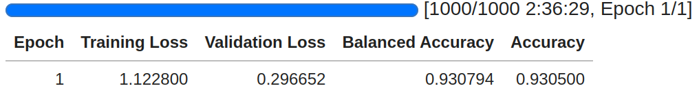
• Above, we test that the coaching has taken place for 1000 steps. It is because we now have 8000 coaching information, and every time, in every step, we ship 8 samples; therefore we now have a complete of 1000 steps
• The coaching came about for two hours and 36 minutes for the mannequin to iterate over the whole coaching information for one epoch
• We will see the coaching lack of the mannequin is 1.12, and the validation loss is 0.29
• The mannequin is displaying a formidable outcome with the validation information, with an accuracy of 93%

Now, allow us to attempt to carry out evaluations to check the newly educated mannequin on the take a look at information:

def generate_predictions(mannequin,df_test):
    sentences = df_test.textual content.tolist()
    batch_size = 32  
    all_outputs = []

    for i in vary(0, len(sentences), batch_size):

        batch_sentences = sentences[i:i + batch_size]

        inputs = tokenizer(batch_sentences, return_tensors="pt", 
        padding=True, truncation=True, max_length=512)

        inputs = {okay: v.to('cuda' if torch.cuda.is_available() else 'cpu') 
        for okay, v in inputs.objects()}

        with torch.no_grad():
            outputs = mannequin(**inputs)
            all_outputs.append(outputs['logits'])
        
    final_outputs = torch.cat(all_outputs, dim=0)
    df_test['predictions']=final_outputs.argmax(axis=1).cpu().numpy()

generate_predictions(mannequin,test_df)
get_performance_metrics(test_df)

Code Rationalization

• Right here, we create a perform similar to the one which we now have created
• On this perform, we convert the textual content column from the take a look at dataframe into a listing of sentences after which run a for loop with a step measurement equal to the batch measurement
• On this for loop, we take the batch variety of sentences, ship them to the tokenizer to tokenize them, and push them to the GPU
• Then, we insert this listing of tokens into the mannequin and get the listing of chances from it
• Lastly, we get the index of the best chance in every output and save the index again within the take a look at dataframe
• This test_df is given again to the get_performance_metric perform which takes on this dataframe and outputs the outcomes

Operating this code has generated the next outcomes. We see that there’s a nice increase within the accuracy of the mannequin. Different metrics like precision, recall, and f1-score have elevated too from their preliminary values. The general accuracy has elevated from 0.23 earlier than coaching to 0.93 after coaching, which is a 0.7 i.e. 70% enchancment within the mannequin after coaching it. From this, we will get an perception that Giant Language Fashions are very a lot able to being employed as sequence classifiers

Conclusion

In conclusion, fine-tuning giant language fashions (LLMs) (finetune Llama 3) for sequence classification includes a number of detailed steps, from getting ready the dataset to quantizing the mannequin for environment friendly coaching on restricted {hardware}. By using varied libraries from HuggingFace and implementing methods reminiscent of Immediate Engineering and LoRA configurations, it’s attainable to successfully practice these fashions for particular duties reminiscent of information classification. This information has demonstrated the whole course of, from preliminary setup and information preprocessing to mannequin coaching and analysis, highlighting the flexibility and energy of LLMs in pure language processing duties.

Key Takeaways

• Giant Language Fashions (finetune Llama 3) are pre-trained on in depth datasets and are able to producing and understanding advanced textual content
• Whereas helpful, immediate engineering alone might not suffice for all classification duties; mannequin fine-tuning can present higher efficiency
• Correctly loading, splitting, and balancing datasets are basic steps earlier than mannequin coaching to make sure correct and honest mannequin efficiency
• Defining customized error metrics and coaching loops is important for dealing with particular necessities like class weights in sequence classification duties
• Pre-training and post-training evaluations utilizing metrics reminiscent of accuracy and balanced accuracy present insights into mannequin efficiency and the effectiveness of the coaching course of

The media proven on this article should not owned by Analytics Vidhya and is used on the Writer’s discretion.